Chapter 20 BCR clonotype analysis

20.1 Processing summary

Fastq files have previously been run through TRUST4 using the Rn6 BCR annotations using the following code (not run here). Note that the bcr/tcr .fa files were assembled using the ensembl annotation (these annotations are not present in the UCSC genomic files). Annotation files for the rn6 BCR regions are available at IMGT, but TCR regions are not available

# obtain the gene names for rat:
library(biomaRt)
human = useEnsembl("ensembl", mirror="useast", dataset = "hsapiens_gene_ensembl")
rat = useEnsembl("ensembl", mirror="useast", data="rnorvegicus_gene_ensembl")
TS = human_igg_trv_list
Hum2RatProt = getLDS(attributes = c("hgnc_symbol", "ensembl_transcript_id"), filters = "hgnc_symbol",  values = TS , mart = human, attributesL = c("rgd_symbol", "ensembl_transcript_id”, “ensemble_gene_id"), martL = rat, uniqueRows=T)
write.table(unique(Hum2RatProt$ensemble_gene_id), "ensbl_rat_bcr.txt", quote=F, row.names=F,colnames=F)

# obtain the tcr/bcr.fa file
#(Note that BuildDatabaseFa.pl needs to be edited on lines 95, 102, 114 and 121 to use transcript_id or gene_id instead)

perl BuildDatabaseFa.pl Rattus_norvegicus.Rnor_6.0.dna_sm.toplevel.fa Rattus_norvegicus.Rnor_6.0.99.gtf ensbl_rat_bcr.txt > bcrtcr_rat_ens.fa

# Obtain the reference annotation file
perl BuildImgtAnnot.pl Rattus_norvegicus > Rnor_IMGT+C.fa

# Run TRUST (below is single end)
./run-trust4 -u 20170125_NMU7_Tumor_RLU_CD45_CGDA5146_S1_R1_001.fastq.gz -f bcrtcr_rat_ens.fa --ref Rnor_IMGT+C.fa

#Annotation file: Load in an annotation file indicating all the samples, batch effects etc 


TRUST4path="../data/TRUST4/"
TRUST4files=dir(TRUST4path,"*.tsv")
#FileNames=sapply(strsplit(TRUST4files, "_report.tsv"), function(x) x[1])
matchidx=match(TRUST4files, infoTableFinal$TRUSTName)

#RepNames=paste(infoTableFinal$Rat_ID, tempAnnot$Location, tempAnnot$Fraction, sep="_")[matchidx]
# load in all the files and save the list to file
RatTrust=lapply(TRUST4files, function(x) read.delim(paste(TRUST4path, x, sep=""), sep="\t"))
names(RatTrust)=infoTableFinal$SampleID[matchidx]


TRUST4path="../data/TRUST4/matchedNormal/"
TRUST4files=dir(TRUST4path,"*.tsv")
#FileNames=sapply(strsplit(TRUST4files, "_report.tsv"), function(x) x[1])
FileNames=paste(substr(TRUST4files, 10, 12), "matchedNMUCD45", sep="_")
RatTrustNormal=lapply(TRUST4files, function(x) read.delim(paste(TRUST4path, x, sep=""), sep="\t"))
names(RatTrustNormal)=FileNames

RatTrust=c(RatTrust, RatTrustNormal)

save(RatTrust, file=sprintf("outputs/Rat_TRUST4_%s.RData", Sys.Date()))

20.2 Summary Stats

Firstly, look at the number of BCR regions which have been identified by TRUST4. In green are the CD45 populations, which as expected appear to have a higher number of clonotypes compared to the epithelial and the double-negative populations (in read and orange).

NSamples=sapply(RatTrust, nrow)
NSamplesCt2=sapply(RatTrust, function(x) length(which(x$X.count>=2)))
NSamplesCDR3comp=sapply(RatTrust, function(x) length(which(x$CDR3aa!="partial")))
NSamplesCDR3compCt2=sapply(RatTrust, function(x) length(which(x$CDR3aa!="partial" & x$X.count>=2)))

TableOut=cbind(NSamples, NSamplesCt2, NSamplesCDR3comp, NSamplesCDR3compCt2)

matchidx=match(rownames(TableOut), infoTableFinal$SampleID)
ColOut=factor(paste(infoTableFinal$Fraction[matchidx], infoTableFinal$Batch[matchidx]))
#palette(c("#e5f5e0","#a1d99b", "#31a354",  "#fd8d3c","#fa9fb5", "#f03b20", "#005824"))

#pdf(sprintf("rslt/TRUST4/BCR_summary_QC_%s.pdf", Sys.Date()), height=5, width = 7)

# plot the clonotype diversity, color-code according to both batch and the sample used
par(mar = c(4, 4, 4, 2),  xpd = TRUE)
barplot(NSamplesCt2+1, las=2,log ='y', ylab = "Number of BCR clonotypes", main="Overview of clonotype diversity (2+ reads)", col=ColOut, cex.names = 0.75)
legend("top", inset = c(-0.5, 0.03),  legend = levels(ColOut),  pch = c(19, 19, 19, 19, 19),  col = c(1:6), horiz = T)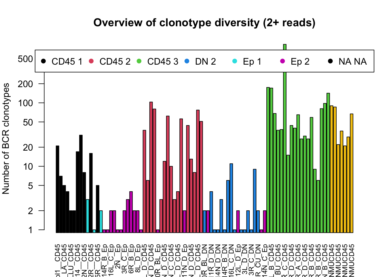

# plot the number of full vs partial clonotypes
PartialvsFull=rbind(NSamplesCDR3compCt2,NSamplesCt2-NSamplesCDR3compCt2)
rownames(PartialvsFull)=c("full", "partial")


par(mar = c(10, 4, 4, 2),  xpd = TRUE)
barplot(PartialvsFull+1, las=2,log ='y', ylab = "Number of BCR clonotypes", main="Proportion of full vs partial CDR3a", col=c(1:2), cex.names = 0.75)
legend("bottom", inset = c(-0.5, -0.5),  legend = c("full", "partial"),  pch = c(19, 19),  col = c(1:2), horiz = T)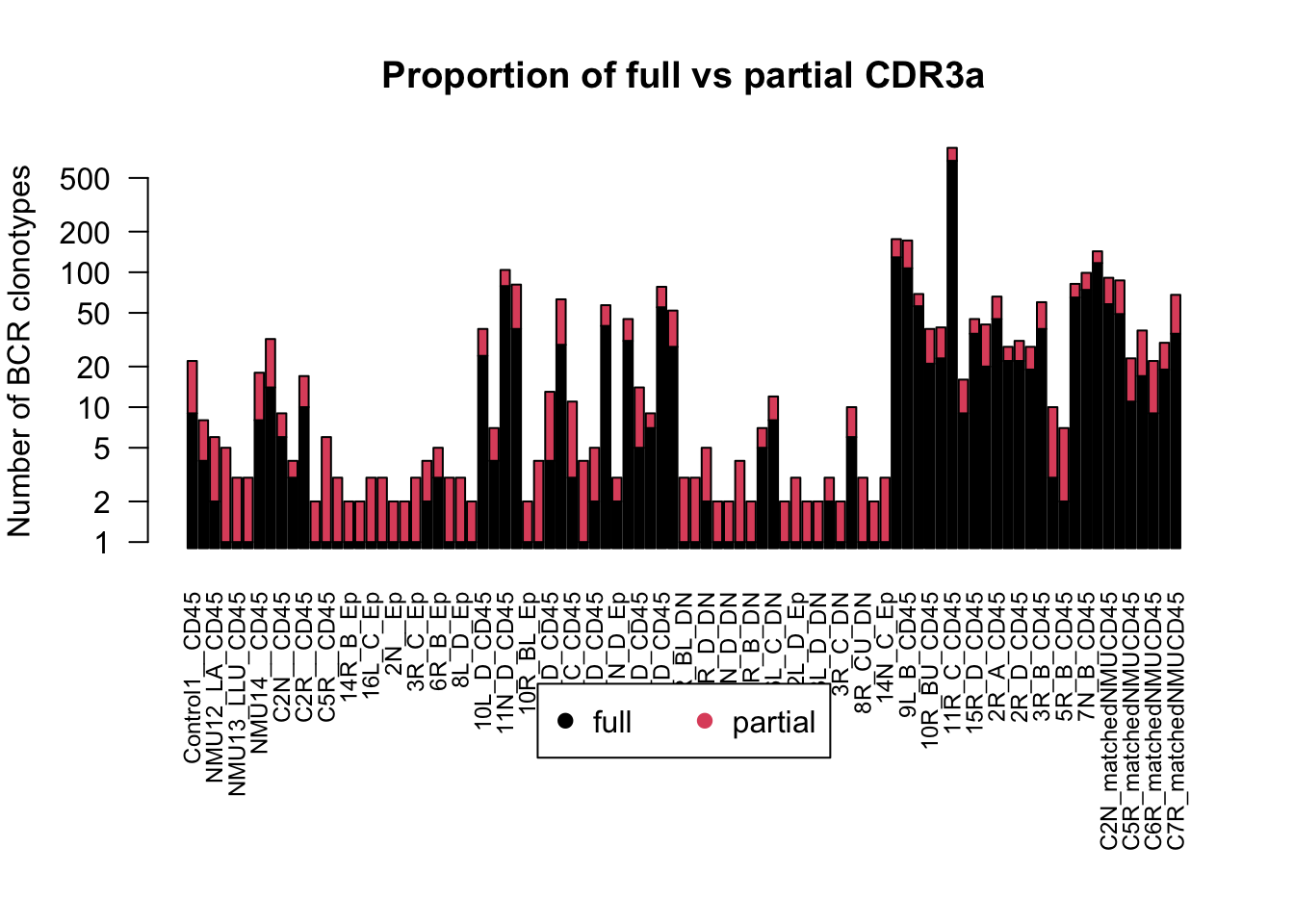

par(mar = c(10, 4, 4, 2),  xpd = TRUE)
barplot(t(TableOut[ which(infoTableFinal$Fraction[matchidx]=="CD45"),]+1), las=2,log ='y', ylab = "Number of BCR clonotypes", main="Clonotype diversity CD45+ samples", col=c(1:4), cex.names = 0.75, beside = T)
legend("bottom", inset = c(-0.5, -0.5),  legend = c("# clonotypes", "clonotypes >2reads", "complete CDR3", "both"),  pch = c(19, 19, 19),  col = c(1:4), horiz = T)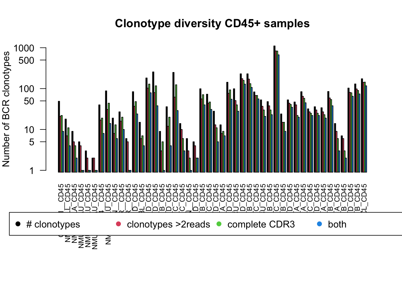

par(mar = c(10, 4, 4, 2),  xpd = TRUE)
barplot(NSamplesCDR3compCt2+1, las=2,log ='y', ylab = "Number of BCR clonotypes", main="Filtered Clonotypes based on batch", col=ColOut, cex.names = 0.75, beside = T)
legend("top", inset = c(-0.5, 0.03),  legend = levels(ColOut),  pch = c(19, 19, 19, 19, 19),  col = c(1:5), horiz = T)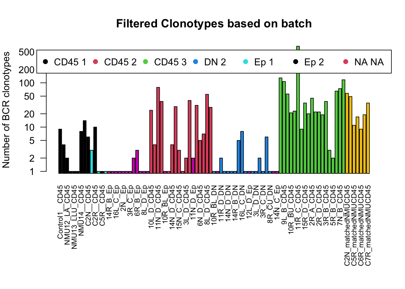

#dev.off()

We will refine the above plot to contain only the CD45 population and assess:

• number of clonotypes
• number of clonotypes with at least 2 reads
• number of clonotypes which have a complete CDR3a region

Note: although this does not look like a big drop, the data is plotted on a log-scale. For example, in the control 4 (first column) a quarter of the clonotypes have at least 2 counts and about half have a complete CDR3 sequence.

For the following analyses, the clonotypes are filtered to only clonotypes with at least 2 supporting reads and a complete VDJ read . When applying this restriction, we have the following distribution of BCR regions. Almost all the epithelial cases do not have supporting reads, and few of the DN cases have supporting reads too.

RatTrustB=lapply(RatTrust, function(x) x[which(x$CDR3aa!="partial" & x$X.count>=2), ])
for (i in 1:length(RatTrustB)){
  RatTrustB[[i]]$frequency=RatTrustB[[i]]$X.count/sum(RatTrustB[[i]]$X.count)
}

20.3 Diversity metrics

We will assess BCR diversity using the following metrics:

** Shannon index **

The shannon index is computed by:

• filtering through reads of interest
• recalculate the fraction such that the new list sums to 1
• compute entropy as the sum of log(freq_x)*freq_x amongst all populations x
• compute the maximum entropy expected for that case -log(1/N), where N is the number of populations present
• to determine confidence intervals, bootstrap the population (500 times) and compute the expected entropy

** Gini index **

The Gini index can be considered as an inverse of the Shannon index

** Top Clonotypes **

We will see the proportion of the BCR repertoire which is computed using the top 10 frequent clones. This will give an idea of whether there is a clonal expansion

# compute values here
Div1=sapply(RatTrustB, function(x) -sum(x$frequency*log(x$frequency), na.rm=T))
EDiv=sapply(NSamplesCDR3compCt2, function(x) -log(1/x))
NormDiv=Div1/EDiv

## Shannon index
# bootstrap rslt
BSrslt=sapply(RatTrustB, function(x) tryCatch(BootstrapShannonIdx(x[ ,1], 1000), error=function(e) c(NA, NA)))
# divide the CI by the maximum possible diversity

BSCI=t(BSrslt)/EDiv

df=data.frame(sample=rownames(BSCI), Val=NormDiv, Lower=BSCI[ , 1], Upper=BSCI[ ,2 ], Type=infoTableFinal$Fraction[matchidx], Batch=infoTableFinal$Batch[matchidx])

## Gini index

Gini=sapply(RatTrustB, function(x) gini(x$frequency))

PGini=sapply(RatTrustB, function(x) tryCatch(PermuteGini(x$X.count, 1000), error=function(e) c(NA, NA)))

df$Calc="shannon"

df2=data.frame(sample=df$sample, Val=Gini, Lower=PGini[1, ], Upper=PGini[2, ], Type=df$Type, Batch=df$Batch,
               Calc="Gini")

dfAll=rbind(df, df2)

## Top Clonotypes

TopClones=sapply(RatTrustB, function(x) sum(x$frequency[1:5], na.rm = T))
TopClones[which(NSamplesCDR3compCt2==0)]=0
df2$Val=TopClones
df2$Calc="Top10"
df2$Lower=TopClones
df2$Upper=TopClones

dfAll=rbind(dfAll, df2)

dfAll$Batch=as.character(dfAll$Batch)
dfAll$Batch[grep("matchedNMU", rownames(dfAll))]="match"
dfAll$Type[grep("matchedNMU", rownames(dfAll))]="CD45"
#ggplot(df[df$Type=="CD45", ], aes(x=sample, y=Val, fill=Type))+geom_bar(stat="identity")+facet_grid(~Batch, scales="free_x", space="free")+geom_errorbar( aes(ymin=Lower, ymax=Upper), width=.2)+theme(axis.text.x = element_text(angle = 90, hjust = 1))+ggtitle("Shannon idx of BCR diversity")

The following plot demonstrates the relationship between the above metrics

#pdf(sprintf("rslt/TRUST4/summary_Scores_diversity_%s.pdf", Sys.Date()), width=7, height=5)

ggplot(dfAll[dfAll$Type=="CD45", ], aes(x=sample, y=Val, fill=Type))+geom_bar(stat="identity")+facet_grid(Calc~Batch, scales="free_x", space="free")+geom_errorbar( aes(ymin=Lower, ymax=Upper), width=.2)+theme(axis.text.x = element_text(angle = 90, hjust = 1))+ggtitle("BCR diversity across samples")+ylab("index value")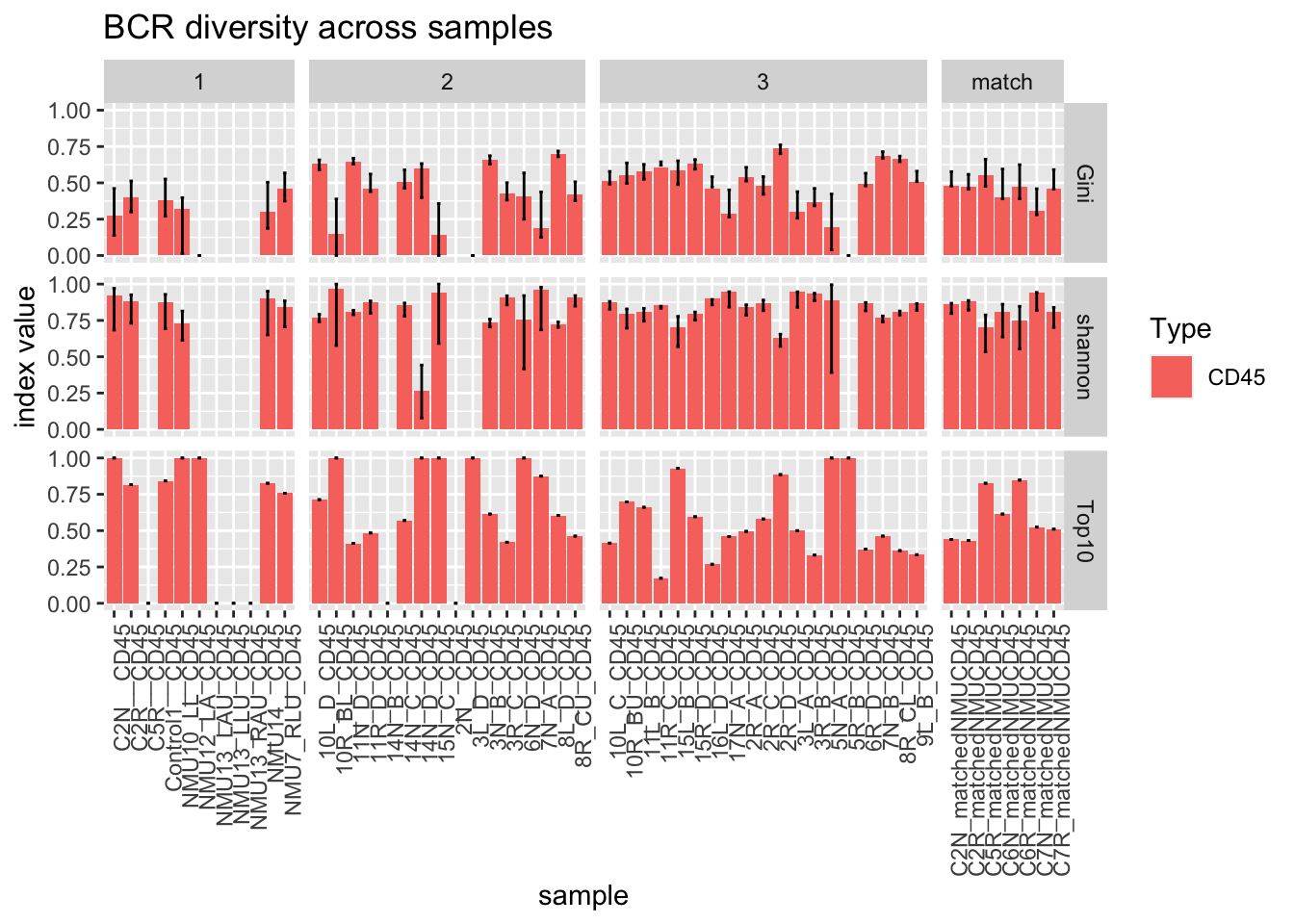

#dev.off()

Notice that some samples have very few clones. An example is 5RB which is represented by a single clonotype, accounting for the absence of a Gini or shannon index

20.4 Compare the characterisation cohort

In the characterisation cohort, we have 3 cases which have CD45 samples in both the tumor and a matched NMU treated mammary gland.

Is there a difference in the clonotypes between these samples?

CharTemp=dfAll[which(dfAll$Type=="CD45" & dfAll$Batch%in%c("1", "match")), ]
CharTemp$Batch[grep("Control", CharTemp$sample)]="Normal"
Nclonotypes=TableOut[which(rownames(TableOut)%in%CharTemp$sample), ]
Nclonotypes2=melt(Nclonotypes)
Nclonotypes2$Case="tumor"
Nclonotypes2$Case[grep("match", Nclonotypes2$Var1)]="mammary"
Nclonotypes2$Case[grep("Control", Nclonotypes2$Var1)]="control"

#pdf(sprintf("rslt/TRUST4/compare_mammary_vs_tumor_%s.pdf", Sys.Date()), width=8, height=6)
a1=sapply(unique(CharTemp$Calc), function(x) wilcox.test(CharTemp$Val[CharTemp$Calc==x & CharTemp$Batch==1], CharTemp$Val[CharTemp$Calc==x & CharTemp$Batch=="match"])$p.value)
p=ggplot(CharTemp, aes(x=Batch, y=Val))+geom_boxplot()+facet_grid(~Calc)+ggtitle(sprintf("wilcox pval: Gini %s, Shannon %s, Top10 = %s", round(a1[2],2), round(a1[1],2), round(a1[3],2)))+geom_jitter(col="grey")+theme_bw()
print(p)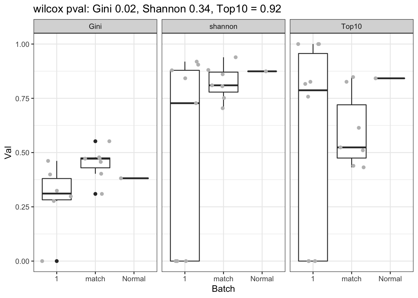

Figure 20.1: bcr clonotypes in tumor and normal mammary glands

#write.csv(CharTemp, file="nature-tables/2h.csv")

DT::datatable(CharTemp, rownames=F, class='cell-border stripe',
          extensions="Buttons", options=list(dom="Bfrtip", buttons=c('csv', 'excel')))

Figure 20.1: bcr clonotypes in tumor and normal mammary glands

Next, we check whether this could be attributed to the total number of clones. Here is a plot which assesses whether these are similar or different

a1=sapply(unique(Nclonotypes2$Var2), function(x) wilcox.test(Nclonotypes2$value[Nclonotypes2$Var2==x & Nclonotypes2$Case=="tumor"], 
                                                             Nclonotypes2$value[Nclonotypes2$Var2==x & Nclonotypes2$Case=="mammary"])$p.value)

ann_text2 <- data.frame(lab=paste("p=", round(a1,4),sep=""), Var2=unique(Nclonotypes2$Var2), Case=1, value=2)
p=ggplot(Nclonotypes2, aes(x=Case, y=value))+geom_boxplot()+facet_grid(~Var2)+ggtitle("Nclonotype with different filters")+geom_jitter(col="grey")+theme_bw()+
  geom_text(data=ann_text2, aes(label=lab))
print(p)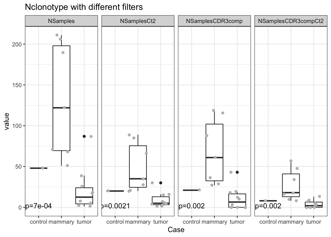

What about association with size?

CharTemp2=CharTemp[which(CharTemp$Batch=="1"), ]
midx=Cdata$Tumor.diameter.sac.mm[match(substr(as.character(CharTemp2$sample), 1, nchar(as.character(CharTemp2$sample))-5), Cdata$TumorID)]
CharTemp2$size=midx


ggplot(CharTemp2, aes(x=size, y=Val))+geom_point()+facet_grid(~Calc)+theme_bw()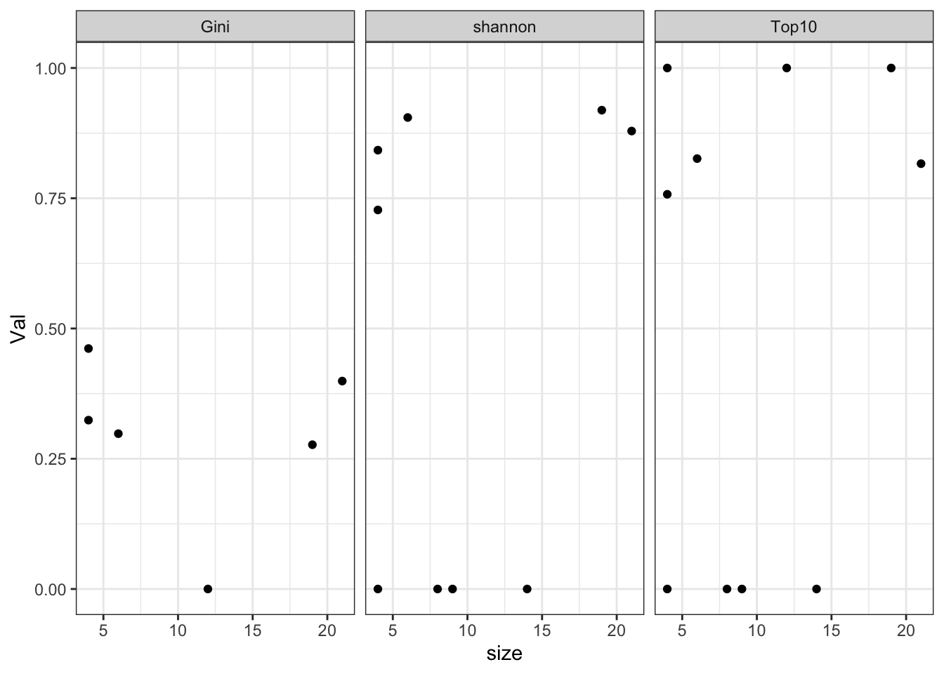

Figure 20.2: clonotype assoc with size

#write.csv(CharTemp2, file="nature-tables/Ext2e.csv")
DT::datatable(CharTemp2, rownames=F, class='cell-border stripe',
          extensions="Buttons", options=list(dom="Bfrtip", buttons=c('csv', 'excel')))

Figure 20.2: clonotype assoc with size

ProgTemp=dfAll[which(dfAll$Type=="CD45" & dfAll$sample%in%infoTableFinal$SampleID[which(infoTableFinal$Cohort=="Progression")]), ]
a1=match(ProgTemp$sample, infoTable)
ProgTemp$Growth=infoTableFinal$Growth[a1]
ProgTemp$NewID=infoTableFinal$TumorIDnew[a1]
ProgTemp$Treatment=infoTableFinal$Treatment[a1]

Nclonotypes=TableOut[which(rownames(TableOut)%in%ProgTemp$sample), ]
Nclonotypes2=melt(Nclonotypes)
# Nclonotypes2$Case="tumor"
# Nclonotypes2$Case[grep("match", Nclonotypes2$Var1)]="mammary"
# Nclonotypes2$Case[grep("Control", Nclonotypes2$Var1)]="control"


head(Nclonotypes2)
#pdf(sprintf("rslt/TRUST4/compare_mammary_vs_tumor_%s.pdf", Sys.Date()), width=8, height=6)
#a1=sapply(unique(ProgTemp$Calc), function(x) wilcox.test(ProgTemp$Val[ProgTemp$Calc==x & ProgTemp$Batch==1], ProgTemp$Val[ProgTemp$Calc==x & ProgTemp$Batch=="match"])$p.value)

p=ggplot(ProgTemp, aes(x=Growth, y=Val))+geom_boxplot()+facet_grid(~Calc)+ggtitle(sprintf("wilcox pval: Gini %s, Shannon %s, Top10 = %s", round(a1[2],2), round(a1[1],2), round(a1[3],2)))+geom_jitter(col="grey")+theme_bw()
print(p)

DT::datatable(ProgTemp, rownames=F, class='cell-border stripe',
          extensions="Buttons", options=list(dom="Bfrtip", buttons=c('csv', 'excel')))

#write.csv(ProgTemp, file="nature-tables/4i_clonotypes.csv")


# a1=sapply(unique(Nclonotypes2$Var2), function(x) wilcox.test(Nclonotypes2$value[Nclonotypes2$Var2==x & Nclonotypes2$Case=="tumor"], Nclonotypes2$value[Nclonotypes2$Var2==x & Nclonotypes2$Case=="mammary"])$p.value)
# 
# ann_text2 <- data.frame(lab=paste("p=", round(a1,4),sep=""), Var2=unique(Nclonotypes2$Var2), Case=1, value=2)
# p=ggplot(Nclonotypes2, aes(x=Case, y=value))+geom_boxplot()+facet_grid(~Var2)+ggtitle("Nclonotype with different filters")+geom_jitter(col="grey")+theme_bw()+
#   geom_text(data=ann_text2, aes(label=lab))
# print(p)

20.5 Associate with clinicopathological data (progression)

We will associate the following metrics:

• total unique clones
• diversity

with the following immune data:

• CD45 fraction (from FACS)
• CD8 fraction (from WSI)
• MH-mixing indices
• Tumor Size
• Growth
• Treatment

matchidx=match(rownames(TableOut), infoTableFinal$SampleID)

TrustTab=infoTableFinal[matchidx, ]

TrustTab$TrustNclonotypes=TableOut[match(TrustTab$SampleID, rownames(TableOut)) ,2]
TrustTab$TrustShannon=dfAll$Val[match(TrustTab$SampleID, dfAll$sample) ]
TrustTab$TrustTop10=df2$Val[match(TrustTab$SampleID, df2$sample)]
TrustTab$TrustGini=dfAll$Val[which(dfAll$Calc=="Gini")[match(TrustTab$SampleID, dfAll$sample)] ]
TrustTab$CD45FACS=as.numeric(as.character(Cdata$CD45.Frac.FACS[match(TrustTab$TumorID, Cdata$TumorID)]))
TrustTab$UnclassFrac=as.numeric(as.character(Cdata$UnclassFraction[match(TrustTab$TumorID, Cdata$TumorID)]))
CD45F=which(TrustTab$Fraction=="CD45")
#TrustTab=TrustTab[TrustTab$Fraction=="CD45", ]

paramSearch=c("CD8Frac", "TumSize", "CD45FACS", "MHEpCAM", "MHSMA", "IFEpCAM", "IFSMA", "UnclassFrac")
FeatTrust=c("TrustNclonotypes", "TrustShannon", "TrustGini", "TrustTop10")

Nclon=sapply(paramSearch, function(x) cor.test(TrustTab[CD45F ,x], TrustTab[ CD45F,c("TrustNclonotypes")], use="complete", method="spearman")$p.value)
SDiv=sapply(paramSearch, function(x) cor.test(TrustTab[CD45F ,x], TrustTab[CD45F ,c("TrustShannon")], use="complete", method="spearman")$p.value)
GDiv=sapply(paramSearch, function(x) cor.test(TrustTab[ CD45F,x], TrustTab[CD45F ,c("TrustGini")], use="complete", method="spearman")$p.value)
TDiv=sapply(paramSearch, function(x) cor.test(TrustTab[CD45F ,x], TrustTab[CD45F ,c("TrustTop10")], use="complete", method="spearman")$p.value)

AllSmerge=rbind(Nclon, SDiv, GDiv, TDiv)

#pdf(sprintf("rslt/TRUST4/association_trustmetrics_clinicopathological_%s.pdf", Sys.Date()), width=10, height=8)

heatmap.2(AllSmerge, scale="none", col=RdBu[11:1], trace="none", main="p values of associations")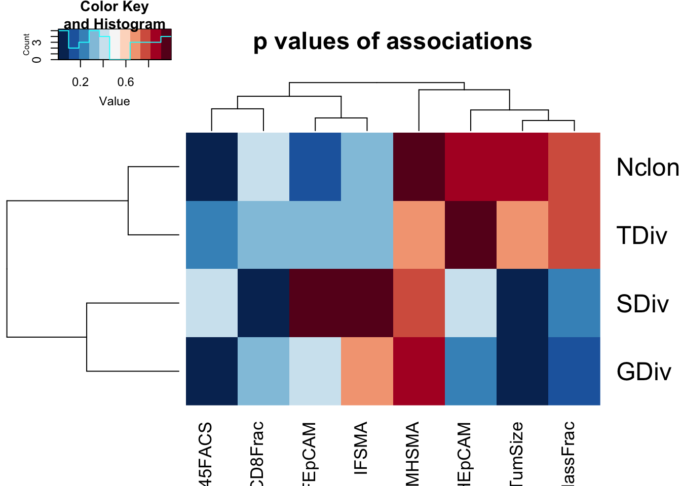

Figure 20.3: 4i: trust result

par(mfrow=c(2,2))
idx=which(AllSmerge<0.1, arr.ind=T)
for (i in 1:nrow(idx)){
  a1=cor.test(TrustTab[CD45F , FeatTrust[idx[i, 1]]]  ,TrustTab[CD45F , paramSearch[idx[i, 2]]], use="complete", method="spearman")
  plot(TrustTab[CD45F , FeatTrust[idx[i, 1]]]  ,TrustTab[CD45F , paramSearch[idx[i, 2]]], xlab=FeatTrust[idx[i, 1]], ylab=paramSearch[idx[i, 2]],
       main=sprintf("cor:%s p:%s", round(a1$estimate,2), round(a1$p.value,2)))
  text(TrustTab[CD45F , FeatTrust[idx[i, 1]]]  ,TrustTab[CD45F , paramSearch[idx[i, 2]]], rownames(TrustTab)[CD45F], cex=0.75)
}

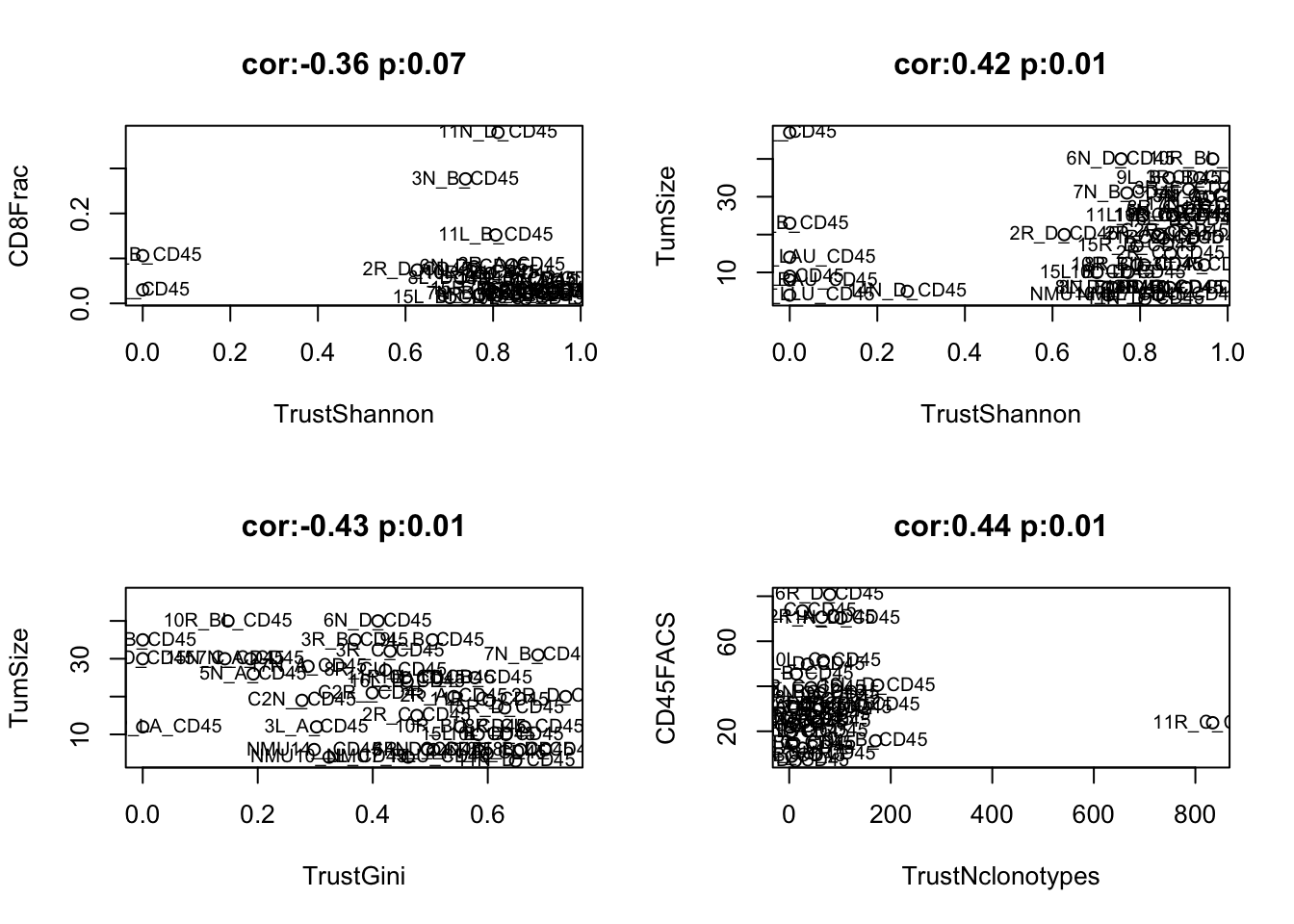
Figure 20.4: 4i: trust result

#pdf("~/Desktop/4L-TRUST-rslt-associate-outcome-progression.pdf", height=8, width=8)

CD45F2=which(TrustTab$Fraction=="CD45" & TrustTab$Cohort=="Progression")

yvals=c("TrustNclonotypes", "TrustShannon", "TrustGini", "TrustTop10")
## associate with growth and treatment type
par(mfrow=c(2,2))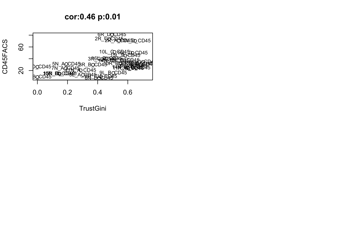

Figure 20.5: 4i: trust result

CD45F2a=which(TrustTab$Fraction=="CD45" & TrustTab$Cohort=="Progression" & 
                TrustTab$Treatment%in%c("Vehicle", "PDL1"))
a1=sapply(yvals, function(x) wilcox.test(TrustTab[CD45F2a ,x]~TrustTab[CD45F2a, "Treatment"])$p.value)
CD45F2a=which(TrustTab$Fraction=="CD45" & TrustTab$Cohort=="Progression" & 
                TrustTab$Treatment%in%c("Vehicle", "LY"))
b1=sapply(yvals, function(x) wilcox.test(TrustTab[CD45F2a ,x]~TrustTab[CD45F2a, "Treatment"])$p.value)
CD45F2a=which(TrustTab$Fraction=="CD45" & TrustTab$Cohort=="Progression" & 
                TrustTab$Treatment%in%c("Vehicle", "PDL1+LY"))
c1=sapply(yvals, function(x) wilcox.test(TrustTab[CD45F2a ,x]~TrustTab[CD45F2a, "Treatment"])$p.value)


TrustTabmelt=melt(TrustTab[CD45F2, ], measure.vars=c("TrustNclonotypes", 
                                                     "TrustShannon", "TrustGini"))

tablex=TrustTab[CD45F2, c("Treatment", "Growth", "TrustNclonotypes", 
                          "TrustShannon", "TrustTop10", "TrustGini")]
tablexM=melt(tablex)

ggplot(tablexM, aes(x=Treatment, y=value, col=Treatment))+geom_boxplot()+geom_point()+facet_wrap(~variable, scales="free")+scale_colour_manual(values=c(ColMerge[ ,1], "black"))+theme_bw()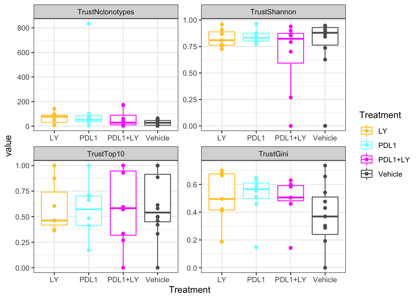

Figure 20.6: trust treatment

#write.csv(tablexM, file="nature-tables/4i_trust-treatment.csv")
DT::datatable(tablexM, rownames=F, class='cell-border stripe',
          extensions="Buttons", options=list(dom="Bfrtip", buttons=c('csv', 'excel')))

Figure 20.6: trust treatment

print('P values PDL1')
## [1] "P values PDL1"
a1
## TrustNclonotypes     TrustShannon        TrustGini       TrustTop10 
##       0.07565166       0.76182641       0.14827564       0.75673324
print('P values LY')
## [1] "P values LY"
b1
## TrustNclonotypes     TrustShannon        TrustGini       TrustTop10 
##       0.06908261       0.73961333       0.23880663       0.73419223
print('P values PDL1+LY')
## [1] "P values PDL1+LY"
c1
## TrustNclonotypes     TrustShannon        TrustGini       TrustTop10 
##        0.5623927        0.3281335        0.2388066        0.9380125

#pdf("figure-outputs/4I_BCR_clonotypes.pdf", height=8, width=5)

ggplot(tablexM, aes(x=Growth, y=value, col=Growth))+geom_boxplot()+geom_point()+facet_wrap(~variable, scales="free")+scale_colour_manual(values=c(ColSizeb, "black"))+theme_bw()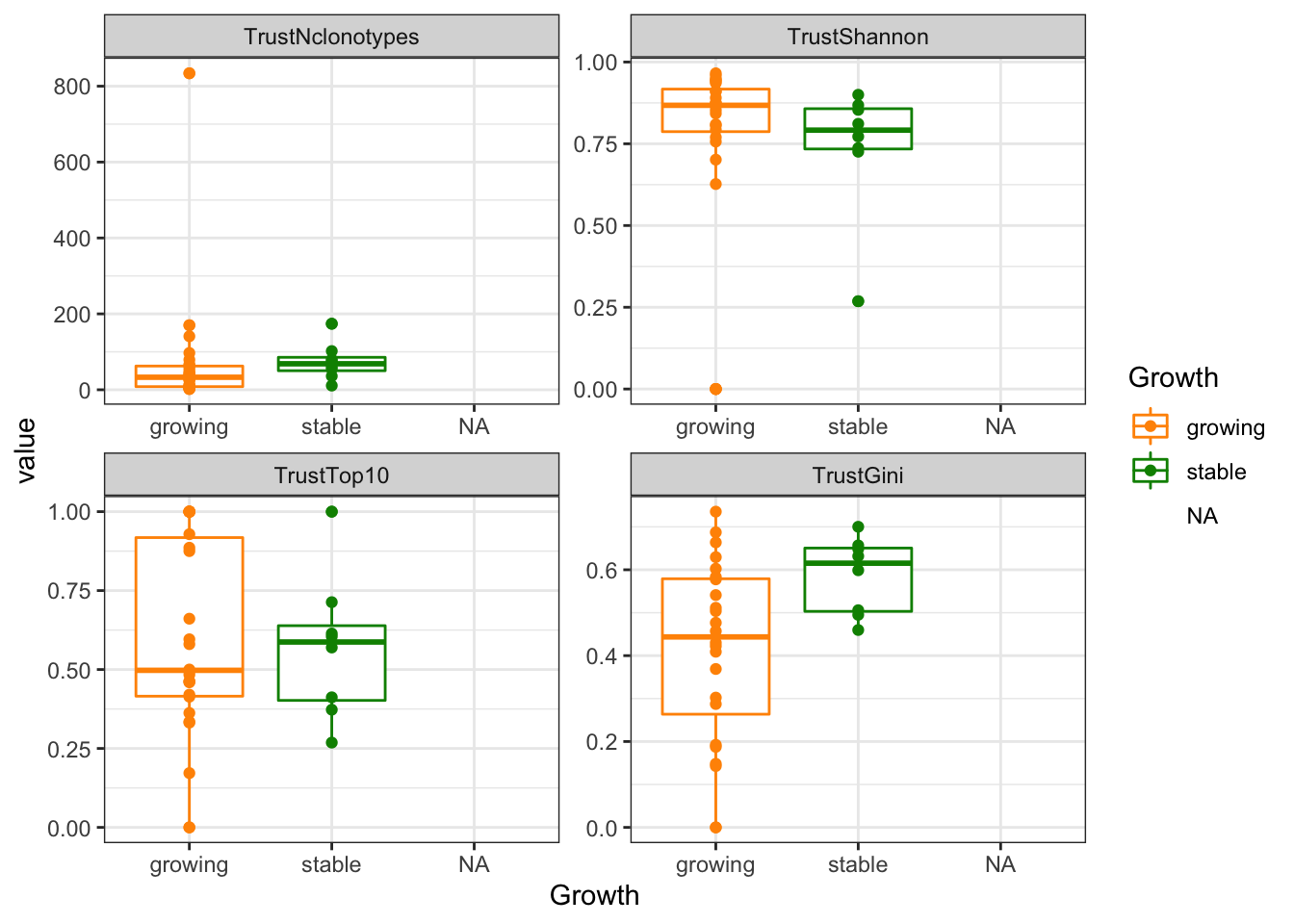

Figure 20.7: trust growth

#dev.off()
#par(mfrow=c(2,2))

a1=sapply(yvals, function(x) wilcox.test(TrustTab[CD45F2 ,x]~TrustTab[CD45F2, "Growth"])$p.value)

print('p values here')
## [1] "p values here"
a1
## TrustNclonotypes     TrustShannon        TrustGini       TrustTop10 
##       0.07072366       0.17037895       0.02795396       0.91880063

20.6 Associate with signature scores

Compare to B cell counts and activation status based on RNA-seq

• B cell signature enrichments scores (from RNA data)

bidx=grep("B cell", output1$cell_type)
idx2=match(TrustTab$SampleID, colnames(output1))

Bsig=output1[bidx, na.omit(idx2)]
rownames(Bsig)=output1$cell_type[bidx]


Bassoc=sapply(FeatTrust, function(y) sapply(1:nrow(Bsig), function(x) cor( t(Bsig[x, ]),(TrustTab[CD45F, y]), use="complete", method="spearman")))
Bassoc2=sapply(FeatTrust, function(y) sapply(1:nrow(Bsig), function(x) cor.test( t(Bsig[x, ]),(TrustTab[CD45F, y]), use="complete", method="spearman")$p.value))
rownames(Bassoc)=rownames(Bsig)

BassocM=Bassoc
BassocM[which(Bassoc2<0.1, arr.ind=T)]=0


#pdf(sprintf("rslt/TRUST4/association_Bcell_signatures_%s.pdf", Sys.Date()), width=7, height=6)
par(oma=c(3, 0,0,5))
heatmap.2(Bassoc, scale="none", trace="none", col=RdBu[11:1], main="correlation")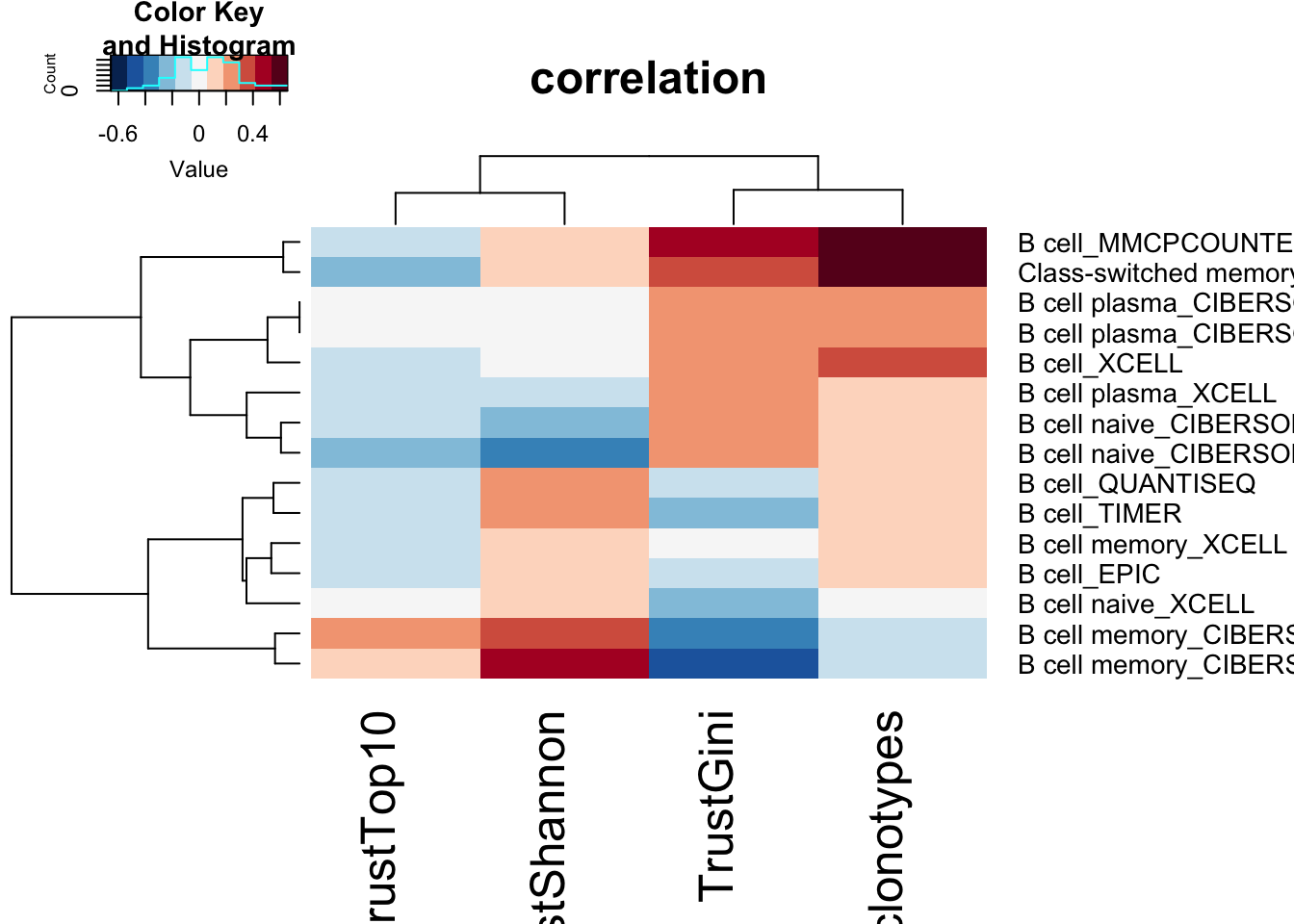

heatmap.2(BassocM, scale="none", trace="none", col=RdBu[11:1], main="significant associations p<0.1 only")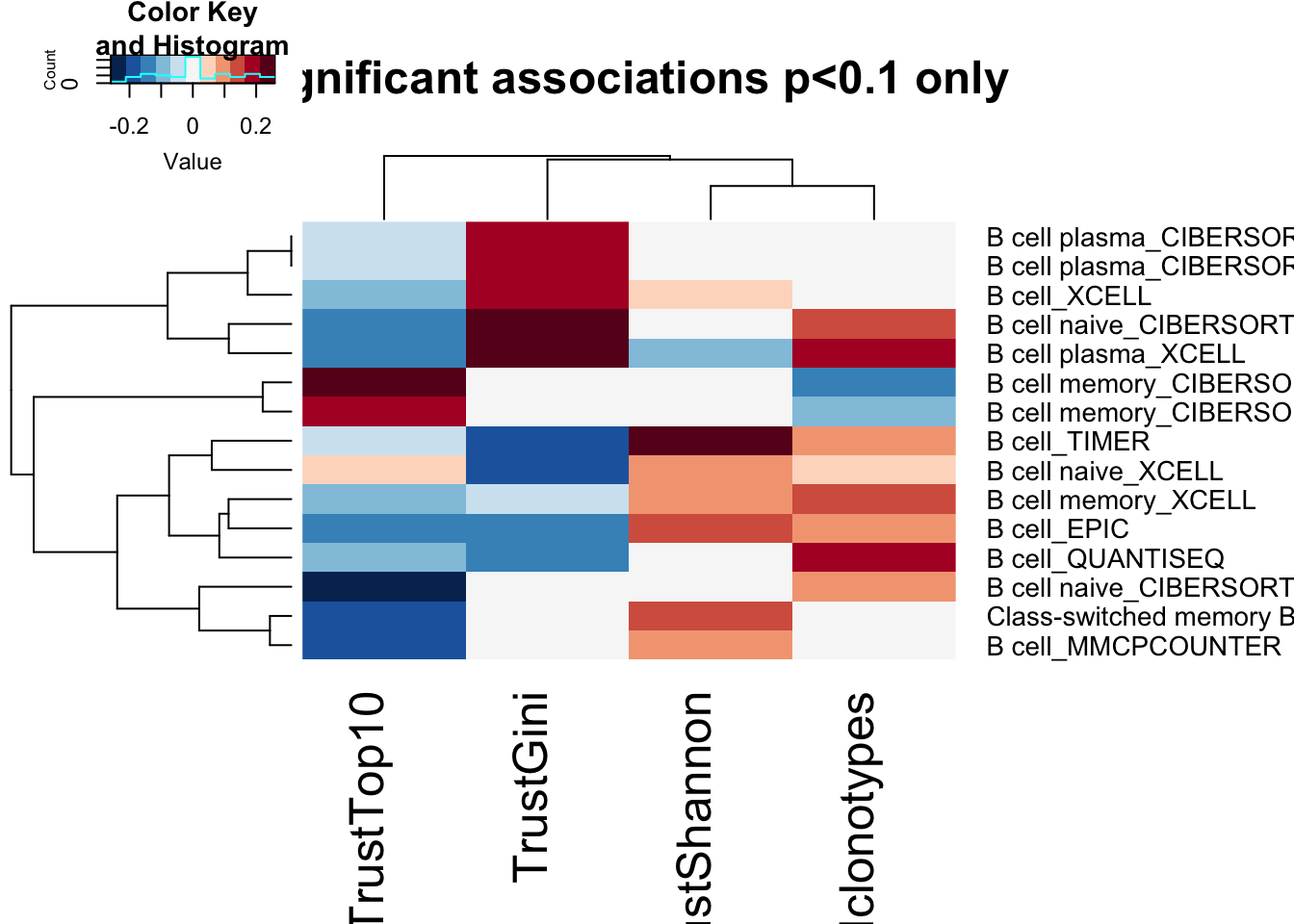

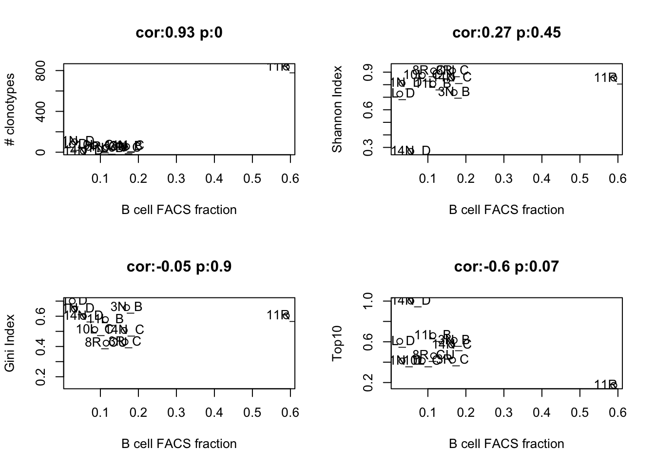
#dev.off()

• B cell frequencies based on FACS:

lx1=match(colnames(Fdata), gsub("_", "", unlist(strsplit( rownames(TrustTab), "_CD45"))))

#pdf(sprintf("rslt/TRUST4/BCR_association_FACS_%s.pdf", Sys.Date()), width=8, height=8)
par(mfrow=c(2,2))
a1=cor.test(as.numeric(t(Fdata[ 9, ])), TrustTab$TrustNclonotypes[lx1], use="complete")
plot(t(Fdata[ 9, ]), TrustTab$TrustNclonotypes[lx1], xlab="B cell FACS fraction", ylab="# clonotypes", main=paste("cor:", round(a1$estimate, 2), " p:", round(a1$p.value,2) ,sep=""))
text(t(Fdata[ 9, ]), TrustTab$TrustNclonotypes[lx1], TrustTab$TumorID[lx1])
a1=cor.test(as.numeric(t(Fdata[ 9, ])), TrustTab$TrustShannon[lx1], use="complete")
plot(t(Fdata[ 9, ]), TrustTab$TrustShannon[lx1], xlab="B cell FACS fraction", ylab="Shannon Index",  main=paste("cor:", round(a1$estimate, 2), " p:", round(a1$p.value,2),sep=""))
text(t(Fdata[ 9, ]), TrustTab$TrustShannon[lx1], TrustTab$TumorID[lx1])
a1=cor.test(as.numeric(t(Fdata[ 9, ])), TrustTab$TrustGini[lx1], use="complete")
plot(t(Fdata[ 9, ]), TrustTab$TrustGini[lx1], xlab="B cell FACS fraction", ylab="Gini Index",  main=paste("cor:", round(a1$estimate, 2), " p:", round(a1$p.value,2),sep=""))
text(t(Fdata[ 9, ]), TrustTab$TrustGini[lx1], TrustTab$TumorID[lx1])
a1=cor.test(as.numeric(t(Fdata[ 9, ])), TrustTab$TrustTop10[lx1], use="complete")
plot(t(Fdata[ 9, ]), TrustTab$TrustTop10[lx1], xlab="B cell FACS fraction", ylab="Top10",  main=paste("cor:", round(a1$estimate, 2), " p:", round(a1$p.value,2),sep=""))
text(t(Fdata[ 9, ]), TrustTab$TrustTop10[lx1], TrustTab$TumorID[lx1])

#dev.off()