Chapter 15 TCGA: Associate Epcam+ inflammatory with survival
Associate the signature with outcome in TCGA: Load in TCGA right now
TCGArsem=read.delim("../data/TCGA/BRCA.rnaseqv2__illuminahiseq_rnaseqv2__unc_edu__Level_3__RSEM_genes_normalized__data.data.txt", sep="\t")
rownames(TCGArsem)=TCGArsem[ ,1]
TCGArsem=TCGArsem[, grep("01A", colnames(TCGArsem))]
colnames(TCGArsem)=substr(colnames(TCGArsem), 1, 12)
colnames(TCGArsem)=gsub("\\.", "-", colnames(TCGArsem))
TCGArsem=TCGArsem[-1, ]

TCGArsem2=apply(TCGArsem, 2, as.numeric)
#TCGArsem2=t(TCGArsem2)
#colnames(TCGArsem2)=colnames(TCGArsem)
#TCGArsem2=data.frame(TCGArsem2)
rownames(TCGArsem2)=rownames(TCGArsem)
rownames(TCGArsem2)=sapply(strsplit(rownames(TCGArsem2), "\\|"), function(x) x[1])
TCGArsem2=TCGArsem2[-which(rownames(TCGArsem2)=="?"), ]

load("../data/TCGA/BrClin_clinical_Nov2017.RData")

ax1=match(BrClin$Patient.ID, colnames(TCGArsem))

BrClin=BrClin[-which(is.na(ax1)), ]
TCGArsem=TCGArsem[ , na.omit(ax1)]

## load in the inflammation subtype information
#ThorssData=read.xlsx("../data/TCGA/Thorsson2018_table1.xlsx",1)
ThorssData=read.csv("../data/TCGA/Thorsson2018_table1.csv")
Edit the clinical data to make sure data is censored at 60 months (5 years) and that stage is given an integer value (no 2A, 2b etc.) for easier comparisons
#m1=match(colnames(TCGAssgsea), BrClin$Patient.ID)
BrClin$Stage=(substr(BrClin$American.Joint.Committee.on.Cancer.Tumor.Stage.Code, 2, 2))
BrClin$Stage[which(BrClin$Stage==""|BrClin$Stage=="X")]=NA

BrClin$Overall.Survival..Months.[which(BrClin$Overall.Survival..Months.>=60)]=60
BrClin$Overall.Survival.Status[which(BrClin$Overall.Survival..Months.>=60)]="LIVING"

BrClin$Disease.Free..Months.[which(BrClin$Disease.Free..Months.>=60)]=60
BrClin$Disease.Free.Status[which(BrClin$Disease.Free..Months.>=60)]="Disease Free"
15.1 Associating CD74 with phenotype and outcome
The Thorsson data has pre-calculated scores for:
- immune subtypes
- leukocyte fractins
- proportion of data with coding mutations
- TCR shannon index
Z-Scale CD74 scores prior to analysis:
TCGAssgsea=scale(TCGArsem2[match("CD74", rownames(TCGArsem2)), ])
m1=match(colnames(TCGArsem2), BrClin$Patient.ID)

tinfo=data.frame(pam=BrClin$PAM50[m1], OSM=BrClin$Overall.Survival..Months.[m1],
                 OSS=BrClin$Overall.Survival.Status[m1], cd74=TCGAssgsea,
                 DFS=BrClin$Disease.Free.Status[m1],
                 DFM=BrClin$Disease.Free..Months.[m1],
                 Stage=BrClin$Stage[m1])

ThorssData=ThorssData[which(ThorssData$TCGA.Study=="BRCA"), ]

n1=match(rownames(tinfo), ThorssData$TCGA.Participant.Barcode)
tinfo$immSub=ThorssData$Immune.Subtype[n1]
tinfo$leukFrac=as.numeric(ThorssData$Leukocyte.Fraction[n1])
tinfo$strFrac=as.numeric(ThorssData$Stromal.Fraction[n1])
tinfo$codingMut=as.numeric(ThorssData$Nonsilent.Mutation.Rate[n1])
tinfo$TCRshann=as.numeric(ThorssData$TCR.Shannon[n1])

par(mfrow=c(2,3))
boxplot(tinfo$cd74~tinfo$pam, ylab="gene exp", main="PAM50")
boxplot(tinfo$cd74~tinfo$immSub, ylab="gene exp", main="Immune sbtype")
ax=cor.test(tinfo$cd74, log10(tinfo$codingMut+1), method="spearman")
smoothScatter(tinfo$cd74, log10(tinfo$codingMut+1), xlab="gene exp", ylab="log10 mut")
text(4,0.5, sprintf("cor=%s, p=%s", round(ax$estimate, 2), round(ax$p.value, 3)))
ax=cor.test(tinfo$cd74, tinfo$leukFrac, method="spearman")
smoothScatter(tinfo$cd74, (tinfo$leukFrac), xlab="gene exp", ylab="leuk frac")
text(4,0.2, sprintf("cor=%s, p=%s", round(ax$estimate, 2), round(ax$p.value, 3)))
ax=cor.test(tinfo$cd74, tinfo$TCRshann, method="spearman")
smoothScatter(tinfo$cd74, tinfo$TCRshann, xlab="gene exp", ylab="TCR diversity")
text(4,1, sprintf("cor=%s, p=%s", round(ax$estimate, 2), round(ax$p.value, 3)))
hist(tinfo$cd74)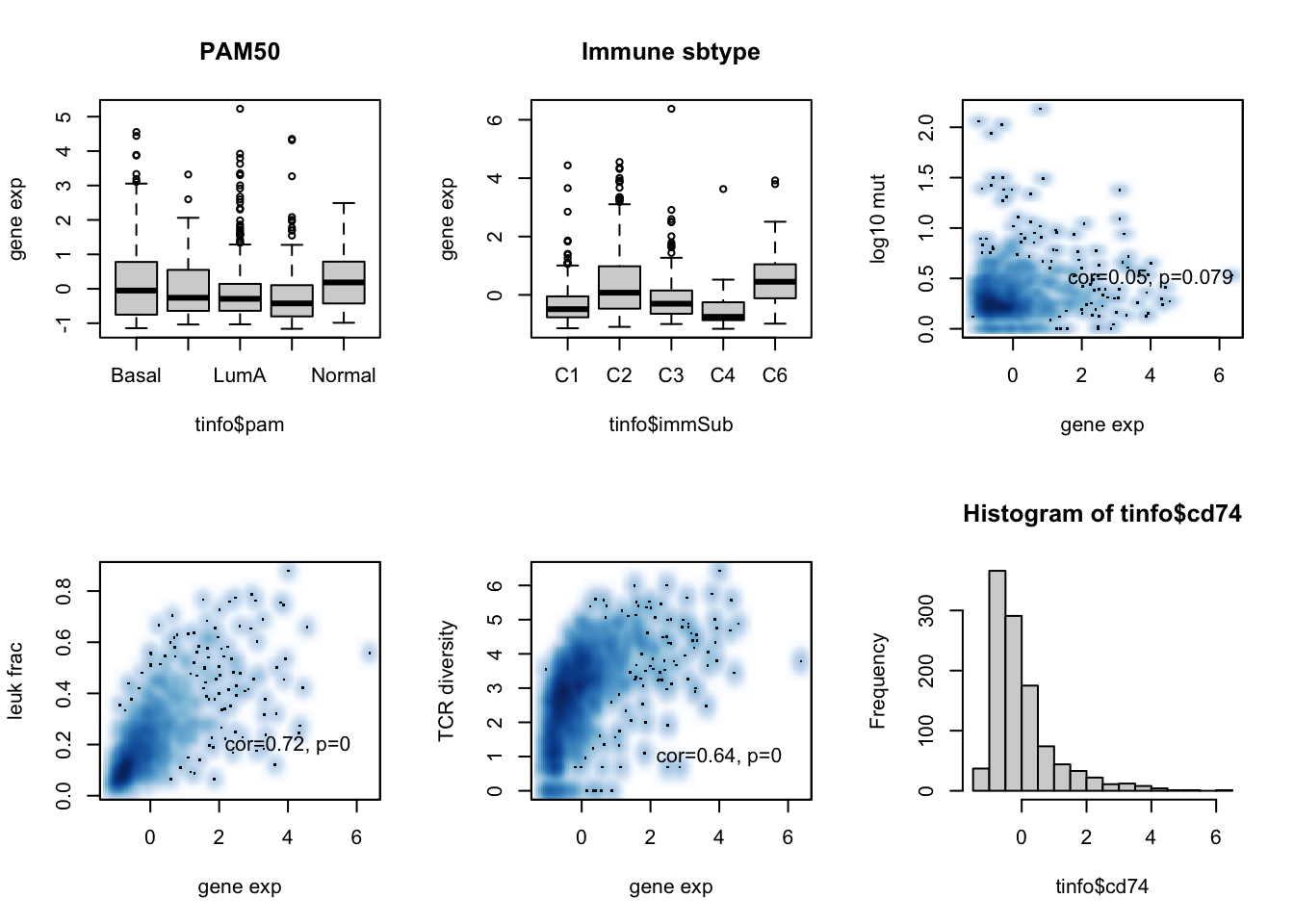
Figure 15.1: CD74 assoc with patient data
We can also check if there is an association with survival:
axD=Surv(tinfo$DFM, ifelse(tinfo$DFS=="Recurred/Progressed", 1, ifelse(tinfo$DFS=="DiseaseFree", 0, NA)))

axO=Surv(tinfo$OSM, ifelse(tinfo$OSS=="DECEASED", 1, ifelse(tinfo$OSS=="LIVING", 0, NA)))

SurvOSS=coxph(axO~tinfo$pam+tinfo$Stage+tinfo$cd74)
SurvDFS=coxph(axD~tinfo$pam+tinfo$Stage+tinfo$cd74)

ao=summary(SurvOSS)
ao
## Call:
## coxph(formula = axO ~ tinfo$pam + tinfo$Stage + tinfo$cd74)
##
##   n= 804, number of events= 78
##    (276 observations deleted due to missingness)
##
##                    coef exp(coef) se(coef)      z Pr(>|z|)
## tinfo$pamHer2    0.3709    1.4491   0.3780  0.981   0.3265
## tinfo$pamLumA   -0.8365    0.4332   0.3091 -2.707   0.0068 **
## tinfo$pamLumB   -0.3137    0.7308   0.3409 -0.920   0.3574
## tinfo$pamNormal -0.2546    0.7752   0.6282 -0.405   0.6853
## tinfo$Stage2     0.6162    1.8519   0.3309  1.862   0.0626 .
## tinfo$Stage3     0.6636    1.9417   0.4315  1.538   0.1241
## tinfo$Stage4     1.9960    7.3594   0.4255  4.691 2.72e-06 ***
## tinfo$cd74      -0.3021    0.7392   0.1530 -1.974   0.0484 *
## ---
## Signif. codes:  0 '***' 0.001 '**' 0.01 '*' 0.05 '.' 0.1 ' ' 1
##
##                 exp(coef) exp(-coef) lower .95 upper .95
## tinfo$pamHer2      1.4491     0.6901    0.6907    3.0400
## tinfo$pamLumA      0.4332     2.3083    0.2364    0.7939
## tinfo$pamLumB      0.7308     1.3685    0.3747    1.4253
## tinfo$pamNormal    0.7752     1.2899    0.2263    2.6557
## tinfo$Stage2       1.8519     0.5400    0.9681    3.5425
## tinfo$Stage3       1.9417     0.5150    0.8335    4.5234
## tinfo$Stage4       7.3594     0.1359    3.1963   16.9448
## tinfo$cd74         0.7392     1.3528    0.5477    0.9978
##
## Concordance= 0.715  (se = 0.031 )
## Likelihood ratio test= 42.32  on 8 df,   p=1e-06
## Wald test            = 47.41  on 8 df,   p=1e-07
## Score (logrank) test = 56.19  on 8 df,   p=3e-09
as=summary(SurvDFS)
as
## Call:
## coxph(formula = axD ~ tinfo$pam + tinfo$Stage + tinfo$cd74)
##
##   n= 587, number of events= 69
##    (493 observations deleted due to missingness)
##
##                    coef exp(coef) se(coef)      z Pr(>|z|)
## tinfo$pamHer2   -0.4626    0.6296   0.4860 -0.952  0.34117
## tinfo$pamLumA   -1.0004    0.3677   0.3158 -3.168  0.00153 **
## tinfo$pamLumB   -0.8377    0.4327   0.3701 -2.263  0.02361 *
## tinfo$pamNormal -0.8810    0.4143   0.7608 -1.158  0.24681
## tinfo$Stage2     0.5470    1.7281   0.3389  1.614  0.10648
## tinfo$Stage3     1.0539    2.8687   0.4440  2.373  0.01762 *
## tinfo$Stage4     2.6058   13.5422   0.4836  5.388 7.13e-08 ***
## tinfo$cd74      -0.1134    0.8928   0.1456 -0.779  0.43600
## ---
## Signif. codes:  0 '***' 0.001 '**' 0.01 '*' 0.05 '.' 0.1 ' ' 1
##
##                 exp(coef) exp(-coef) lower .95 upper .95
## tinfo$pamHer2      0.6296    1.58824   0.24287    1.6323
## tinfo$pamLumA      0.3677    2.71950   0.19802    0.6828
## tinfo$pamLumB      0.4327    2.31113   0.20948    0.8937
## tinfo$pamNormal    0.4143    2.41342   0.09329    1.8404
## tinfo$Stage2       1.7281    0.57866   0.88943    3.3577
## tinfo$Stage3       2.8687    0.34859   1.20151    6.8493
## tinfo$Stage4      13.5422    0.07384   5.24827   34.9432
## tinfo$cd74         0.8928    1.12006   0.67121    1.1876
##
## Concordance= 0.69  (se = 0.039 )
## Likelihood ratio test= 32.15  on 8 df,   p=9e-05
## Wald test            = 39.03  on 8 df,   p=5e-06
## Score (logrank) test = 50.73  on 8 df,   p=3e-08
Note that CD74 is associated with survival: The harzards ratio is 1.851886 (95CI:0.9680967, 3.5424989), p value 1.176905110^{-6}.
This means that this is associated with survival regardless of subtype. We can look at these values in forestplots
data1=data.frame(X1=c("","PAM50", "", "", "", "", "Stage", "","","", "CD74"),
                X2=c("","Basal", "Her2", "LumA", "LumB", "Normal" ,"1", "2", "3", "4", ""),
                X3=c("NSamp",  table(tinfo$pam), table(tinfo$Stage), length(na.omit(tinfo$cd74))),
                X4=c("HR", "", round(summary(SurvOSS)$coefficients[ 1:4,2],2), "",
                     round(summary(SurvOSS)$coefficients[ 5:8,2],2)))

mdata=data.frame(summary(SurvOSS)$conf.int[ ,c(1,3:4)])
mdata=rbind(NA,NA, mdata[1:4, ], NA, mdata[5:8, ])

#pdf("figure-outputs/Figure5_CD74_forestplot.pdf", width=5, height=5)

forestplot(data1, mdata, xlog=T,
           boxsize=0.5)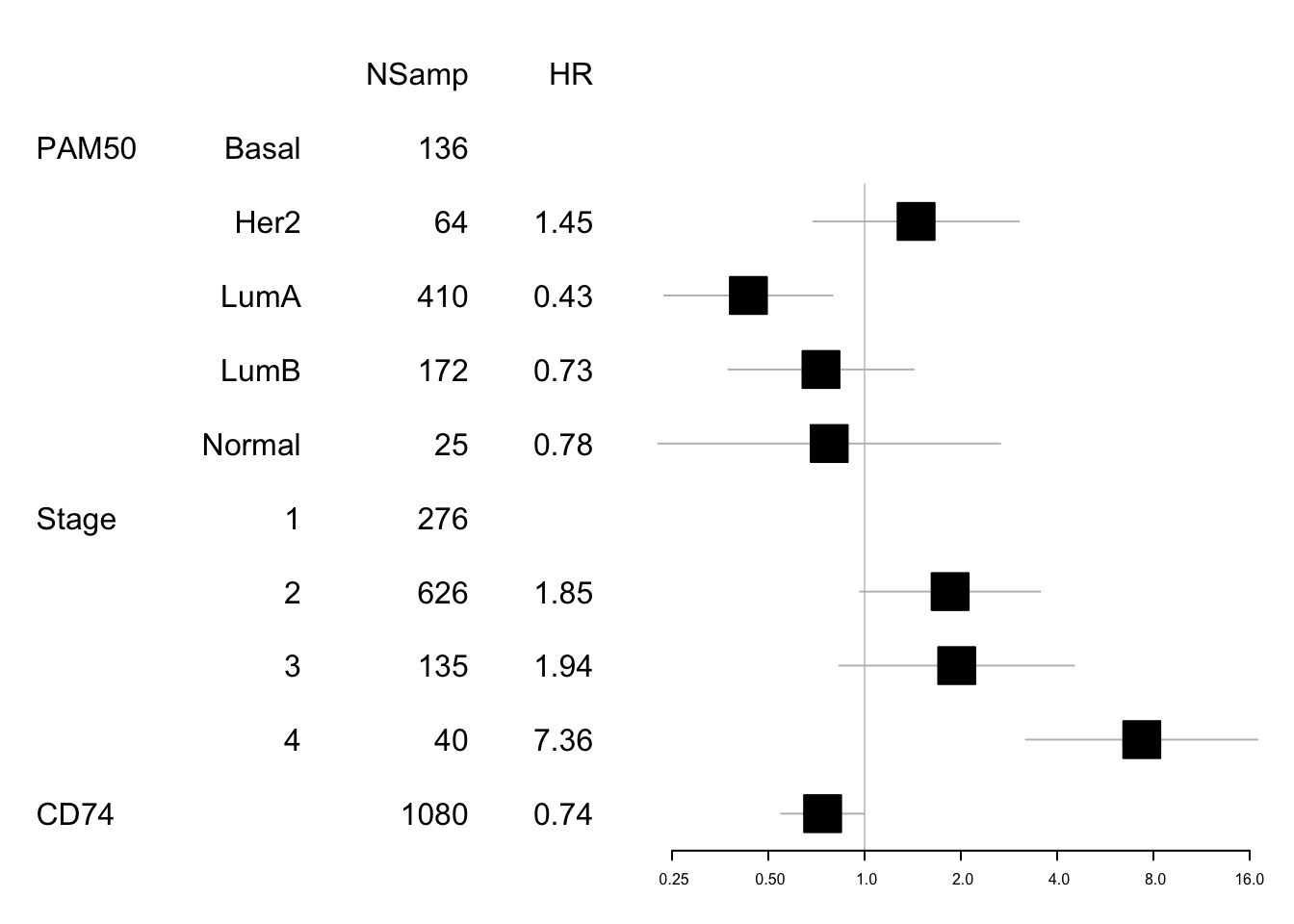
Figure 15.2: forest plot CD74
#write.csv(cbind(data1, mdata), file="nature-tables/5e_forest_plot.csv")

DT::datatable(cbind(data1, mdata), rownames=F, class='cell-border stripe',
          extensions="Buttons", options=list(dom="Bfrtip", buttons=c('csv', 'excel')))
Figure 15.2: forest plot CD74
We can look below what the association with subtype is in KM curves:
par(mfrow=c(2,2))

Xind=c("Basal", "Her2", "LumA", "LumB")

for (i in Xind){
  l1=which(tinfo$pam==i)
  ax=Surv(tinfo$OSM[l1], ifelse(tinfo$OSS[l1]=="DECEASED", 1, ifelse(tinfo$OSS[l1]=="LIVING", 0, NA)))
  TCGAvalCut=cut(tinfo$cd74[l1], quantile(tinfo$cd74[l1], c(0, 0.33, 0.67, 1)), c("L","M", "P"))
  ax1=summary(coxph(ax~TCGAvalCut+tinfo$Stage[l1]))
  ax2=plot(survfit(ax~TCGAvalCut), main=paste(i, "CD74 gene exp"), col=brewer.pal(3, "Blues"),lwd=2, xlab="Time (months)", ylab="OS", mark.time=T)
  text(20, 0.2, sprintf("HR:%s (%s-%s) p=%s", round(ax1$coefficients[2,2 ],2),
                     round(ax1$conf.int[2,3 ],2), round(ax1$conf.int[2, 4],2),round(ax1$logtest[3],2)))
}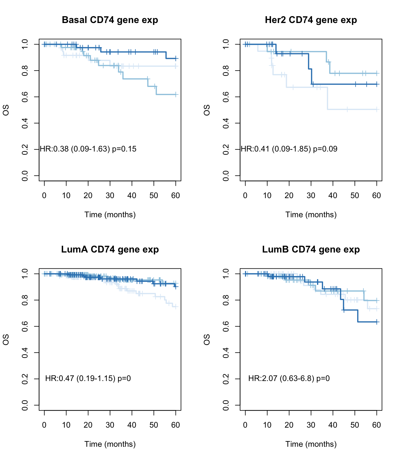
Figure 15.3: OS CD74 by subtype
par(mfrow=c(2,2))

for (i in Xind){
   l1=which(tinfo$pam==i)
  ax=Surv(tinfo$DFM[l1], ifelse(tinfo$DFS[l1]=="Recurred/Progressed", 1, ifelse(tinfo$DFS[l1]=="DiseaseFree", 0, NA)))
  TCGAvalCut=cut(tinfo$cd74[l1], quantile(tinfo$cd74[l1], c(0, 0.33, 0.67, 1)), c("L","M", "P"))
  ax1=summary(coxph(ax~TCGAvalCut+tinfo$Stage[l1]))
  ax2=plot(survfit(ax~TCGAvalCut), main=paste(i, "CD74 gene exp"), col=brewer.pal(3, "Blues"),lwd=2, xlab="Time (months)", ylab="DFS", mark.time=T)
  text(20, 0.2, sprintf("HR:%s (%s-%s) p=%s", round(ax1$coefficients[2,2 ],2),
                     round(ax1$conf.int[2,3 ],2), round(ax1$conf.int[2, 4],2),round(ax1$logtest[3],2)))
}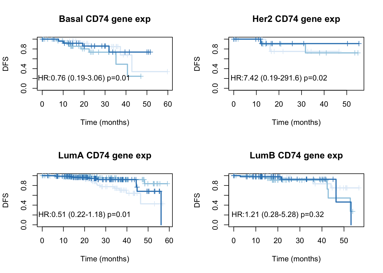
Figure 15.4: DFS CD74 by subtype
15.2 Associating ADMATS10 with phenotype and outcome
Do the same thing as above with the ADAMST10 scores
15.2.1 All samples
Z-Scale ADAMTS10 scores prior to analysis:
TCGAssgsea=scale(TCGArsem2[match("ADAMTS10", rownames(TCGArsem2)), ])
tinfo$adamts10=TCGAssgsea

#pdf("figure-outputs/Figure5_ADAMST10_output.pdf", height=7, width=9)

par(mfrow=c(2,3))
boxplot(tinfo$adamts10~tinfo$pam, ylab="gene exp", main="PAM50")
boxplot(tinfo$adamts10~tinfo$immSub, ylab="gene exp", main="Immune sbtype")
ax=cor.test(tinfo$adamts10, log10(tinfo$codingMut+1), method="spearman")
smoothScatter(tinfo$adamts10, log10(tinfo$codingMut+1), xlab="gene exp", ylab="log10 mut")
text(4,0.5, sprintf("cor=%s, p=%s", round(ax$estimate, 2), round(ax$p.value, 3)))
ax=cor.test(tinfo$adamts10, tinfo$leukFrac, method="spearman")
smoothScatter(tinfo$adamts10, (tinfo$leukFrac), xlab="gene exp", ylab="leuk frac")
text(4,0.2, sprintf("cor=%s, p=%s", round(ax$estimate, 2), round(ax$p.value, 3)))
ax=cor.test(tinfo$adamts10, tinfo$TCRshann, method="spearman")
smoothScatter(tinfo$adamts10, tinfo$TCRshann, xlab="gene exp", ylab="TCR diversity")
text(4,1, sprintf("cor=%s, p=%s", round(ax$estimate, 2), round(ax$p.value, 3)))
#hist(tinfo$adamts10)
ax=cor.test(tinfo$adamts10, tinfo$strFrac, method="spearman")
smoothScatter(tinfo$adamts10, (tinfo$strFrac), xlab="gene exp", ylab="str frac")
text(4,0.2, sprintf("cor=%s, p=%s", round(ax$estimate, 2), round(ax$p.value, 3)))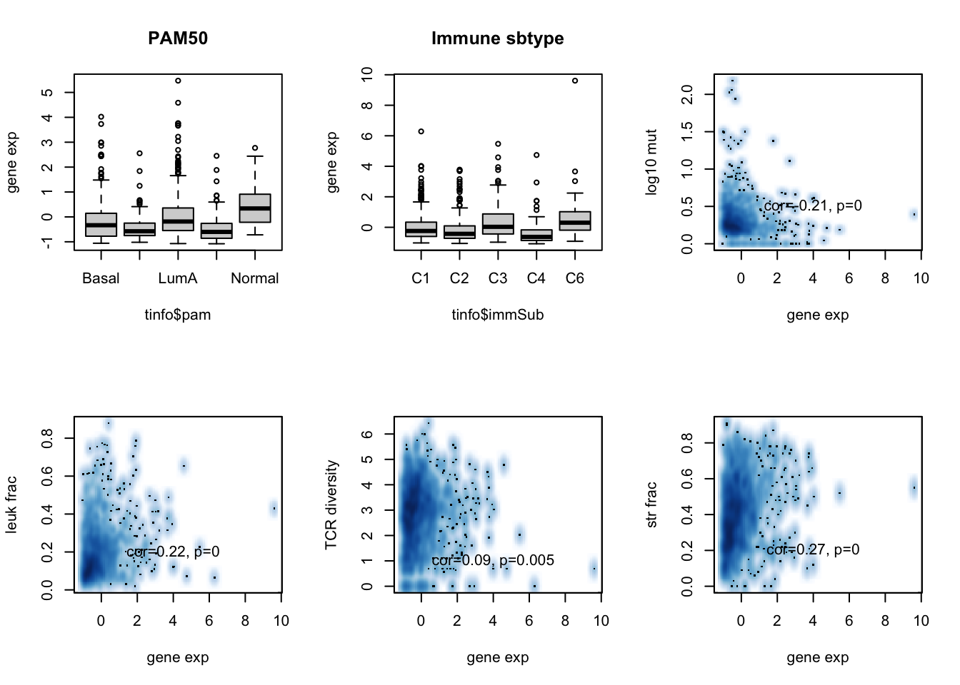
Figure 15.5: ADAMTS10 assoc with patient data
DT::datatable(tinfo, rownames=F, class='cell-border stripe',
          extensions="Buttons", options=list(dom="Bfrtip", buttons=c('csv', 'excel')))
Figure 15.5: ADAMTS10 assoc with patient data
We can also check if there is an association with survival:
axD=Surv(tinfo$DFM, ifelse(tinfo$DFS=="Recurred/Progressed", 1, ifelse(tinfo$DFS=="DiseaseFree", 0, NA)))

axO=Surv(tinfo$OSM, ifelse(tinfo$OSS=="DECEASED", 1, ifelse(tinfo$OSS=="LIVING", 0, NA)))

SurvOSS=coxph(axO~tinfo$pam+tinfo$Stage+tinfo$adamts10)
SurvDFS=coxph(axD~tinfo$pam+tinfo$Stage+tinfo$adamts10)

ao=summary(SurvOSS)
ao
## Call:
## coxph(formula = axO ~ tinfo$pam + tinfo$Stage + tinfo$adamts10)
##
##   n= 804, number of events= 78
##    (276 observations deleted due to missingness)
##
##                     coef exp(coef) se(coef)      z Pr(>|z|)
## tinfo$pamHer2    0.54256   1.72041  0.38290  1.417  0.15649
## tinfo$pamLumA   -0.76154   0.46695  0.30686 -2.482  0.01308 *
## tinfo$pamLumB    0.01904   1.01922  0.34481  0.055  0.95596
## tinfo$pamNormal -0.45045   0.63734  0.62772 -0.718  0.47301
## tinfo$Stage2     0.78659   2.19589  0.32970  2.386  0.01704 *
## tinfo$Stage3     0.65338   1.92203  0.43174  1.513  0.13018
## tinfo$Stage4     2.22438   9.24771  0.42640  5.217 1.82e-07 ***
## tinfo$adamts10   0.33950   1.40424  0.11926  2.847  0.00442 **
## ---
## Signif. codes:  0 '***' 0.001 '**' 0.01 '*' 0.05 '.' 0.1 ' ' 1
##
##                 exp(coef) exp(-coef) lower .95 upper .95
## tinfo$pamHer2      1.7204     0.5813    0.8123    3.6438
## tinfo$pamLumA      0.4669     2.1416    0.2559    0.8521
## tinfo$pamLumB      1.0192     0.9811    0.5185    2.0034
## tinfo$pamNormal    0.6373     1.5690    0.1862    2.1812
## tinfo$Stage2       2.1959     0.4554    1.1507    4.1903
## tinfo$Stage3       1.9220     0.5203    0.8246    4.4798
## tinfo$Stage4       9.2477     0.1081    4.0094   21.3299
## tinfo$adamts10     1.4042     0.7121    1.1116    1.7740
##
## Concordance= 0.705  (se = 0.033 )
## Likelihood ratio test= 44.68  on 8 df,   p=4e-07
## Wald test            = 51.25  on 8 df,   p=2e-08
## Score (logrank) test = 59.87  on 8 df,   p=5e-10
as=summary(SurvDFS)
as
## Call:
## coxph(formula = axD ~ tinfo$pam + tinfo$Stage + tinfo$adamts10)
##
##   n= 587, number of events= 69
##    (493 observations deleted due to missingness)
##
##                    coef exp(coef) se(coef)      z Pr(>|z|)
## tinfo$pamHer2   -0.3174    0.7280   0.4917 -0.646  0.51857
## tinfo$pamLumA   -0.9437    0.3892   0.3139 -3.006  0.00264 **
## tinfo$pamLumB   -0.6459    0.5242   0.3782 -1.708  0.08767 .
## tinfo$pamNormal -1.0680    0.3437   0.7656 -1.395  0.16301
## tinfo$Stage2     0.5881    1.8006   0.3392  1.734  0.08293 .
## tinfo$Stage3     1.0235    2.7830   0.4459  2.295  0.02171 *
## tinfo$Stage4     2.6126   13.6344   0.4816  5.425 5.81e-08 ***
## tinfo$adamts10   0.2219    1.2485   0.1273  1.743  0.08125 .
## ---
## Signif. codes:  0 '***' 0.001 '**' 0.01 '*' 0.05 '.' 0.1 ' ' 1
##
##                 exp(coef) exp(-coef) lower .95 upper .95
## tinfo$pamHer2      0.7280    1.37355   0.27775     1.908
## tinfo$pamLumA      0.3892    2.56954   0.21035     0.720
## tinfo$pamLumB      0.5242    1.90773   0.24978     1.100
## tinfo$pamNormal    0.3437    2.90957   0.07665     1.541
## tinfo$Stage2       1.8006    0.55537   0.92619     3.501
## tinfo$Stage3       2.7830    0.35933   1.16137     6.669
## tinfo$Stage4      13.6344    0.07334   5.30498    35.042
## tinfo$adamts10     1.2485    0.80099   0.97282     1.602
##
## Concordance= 0.671  (se = 0.041 )
## Likelihood ratio test= 34.27  on 8 df,   p=4e-05
## Wald test            = 41.62  on 8 df,   p=2e-06
## Score (logrank) test = 53.32  on 8 df,   p=9e-09
Note that ADAMST10 is associated with survival: The harzards ratio is 2.1958872 (95CI:1.150724, 4.1903363), p value 4.22777410^{-7}.
This means that this is associated with survival regardless of subtype. We can look at these values in forestplots
data1=data.frame(X1=c("","PAM50", "", "", "", "", "Stage", "","","", "ADAMST10"),
                X2=c("","Basal", "Her2", "LumA", "LumB", "Normal" ,"1", "2", "3", "4", ""),
                X3=c("NSamp",  table(tinfo$pam), table(tinfo$Stage), length(na.omit(tinfo$cd74))),
                X4=c("HR", "", round(summary(SurvOSS)$coefficients[ 1:4,2],2), "",
                     round(summary(SurvOSS)$coefficients[ 5:8,2],2)))

mdata=data.frame(summary(SurvOSS)$conf.int[ ,c(1,3:4)])
mdata=rbind(NA,NA, mdata[1:4, ], NA, mdata[5:8, ])

#pdf("figure-outputs/Figure5_CD74_forestplot.pdf", width=5, height=5)

forestplot(data1, mdata, xlog=T,
           boxsize=0.5)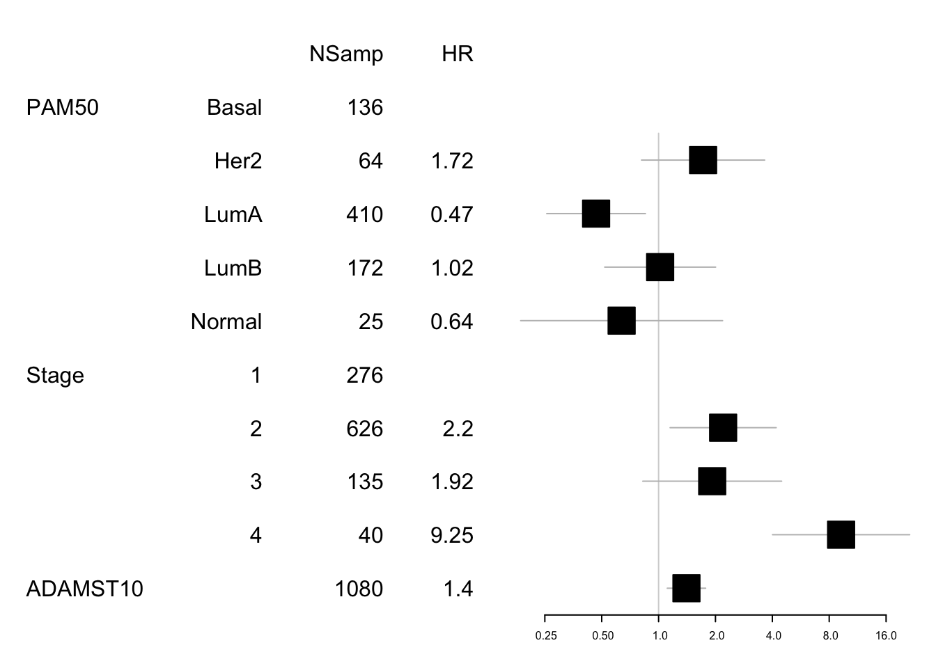
Figure 15.6: forest plot ADAMTS10
#dev.off()
#write.csv(cbind(data1, mdata), file="nature-tables/5e_forest_plot_adamts10.csv")

DT::datatable(cbind(data1, mdata), rownames=F, class='cell-border stripe',
          extensions="Buttons", options=list(dom="Bfrtip", buttons=c('csv', 'excel')))
Figure 15.6: forest plot ADAMTS10
We can look below what the association with subtype is in KM curves:
par(mfrow=c(2,2))

Xind=c("Basal", "Her2", "LumA", "LumB")

for (i in Xind){
  l1=which(tinfo$pam==i)
  ax=Surv(tinfo$OSM[l1], ifelse(tinfo$OSS[l1]=="DECEASED", 1, ifelse(tinfo$OSS[l1]=="LIVING", 0, NA)))
  TCGAvalCut=cut(tinfo$adamts10[l1], quantile(tinfo$adamts10[l1], c(0, 0.33, 0.67, 1)), c("L","M", "P"))
  ax1=summary(coxph(ax~TCGAvalCut+tinfo$Stage[l1]))
  ax2=plot(survfit(ax~TCGAvalCut), main=paste(i, "ADAMTS10 gene exp"), col=brewer.pal(3, "Blues"),lwd=2, xlab="Time (months)", ylab="OS", mark.time=T)
  text(20, 0.2, sprintf("HR:%s (%s-%s) p=%s", round(ax1$coefficients[2,2 ],2),
                     round(ax1$conf.int[2,3 ],2), round(ax1$conf.int[2, 4],2),round(ax1$logtest[3],2)))
}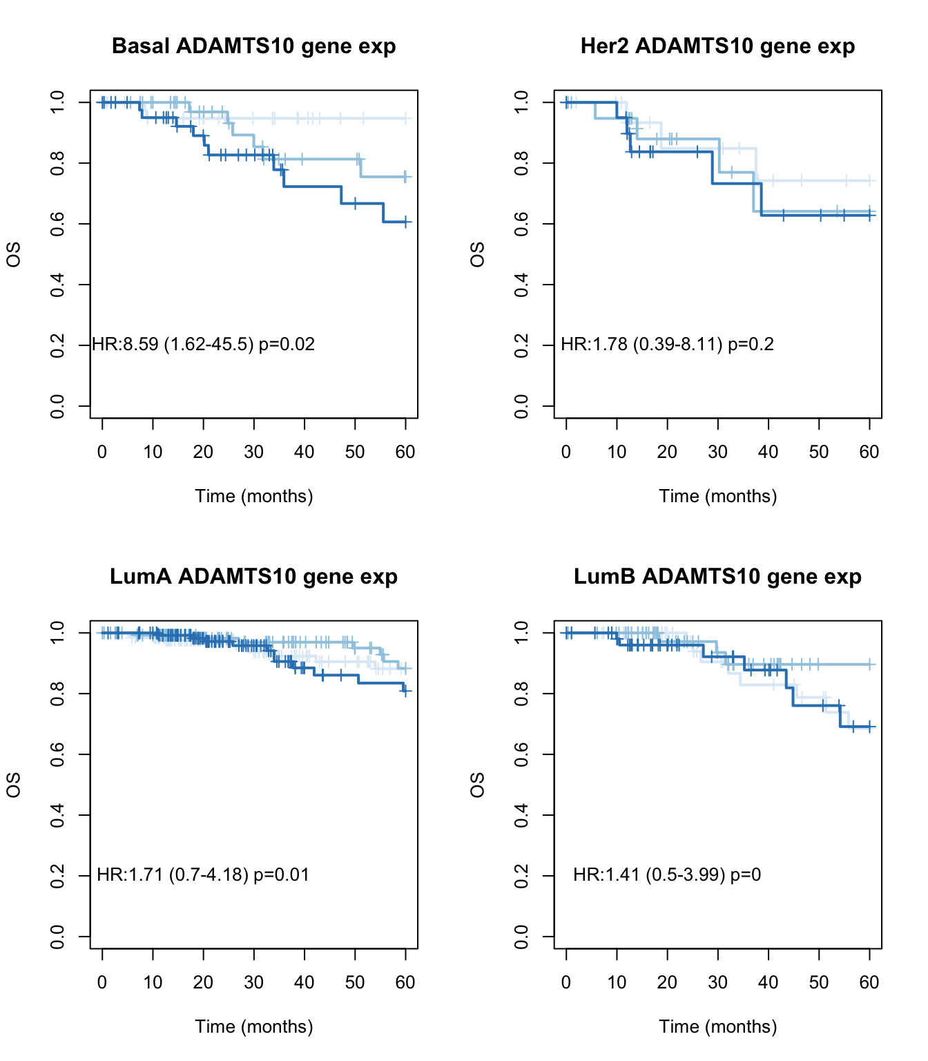
Figure 15.7: OS CD74 by subtype
par(mfrow=c(2,2))

for (i in Xind){
   l1=which(tinfo$pam==i)
  ax=Surv(tinfo$DFM[l1], ifelse(tinfo$DFS[l1]=="Recurred/Progressed", 1, ifelse(tinfo$DFS[l1]=="DiseaseFree", 0, NA)))
  TCGAvalCut=cut(tinfo$adamts10[l1], quantile(tinfo$adamts10[l1], c(0, 0.33, 0.67, 1)), c("L","M", "P"))
  ax1=summary(coxph(ax~TCGAvalCut+tinfo$Stage[l1]))
  ax2=plot(survfit(ax~TCGAvalCut), main=paste(i, "ADAMTS10 gene exp"), col=brewer.pal(3, "Blues"),lwd=2, xlab="Time (months)", ylab="DFS", mark.time=T)
  text(20, 0.2, sprintf("HR:%s (%s-%s) p=%s", round(ax1$coefficients[2,2 ],2),
                     round(ax1$conf.int[2,3 ],2), round(ax1$conf.int[2, 4],2),round(ax1$logtest[3],2)))
}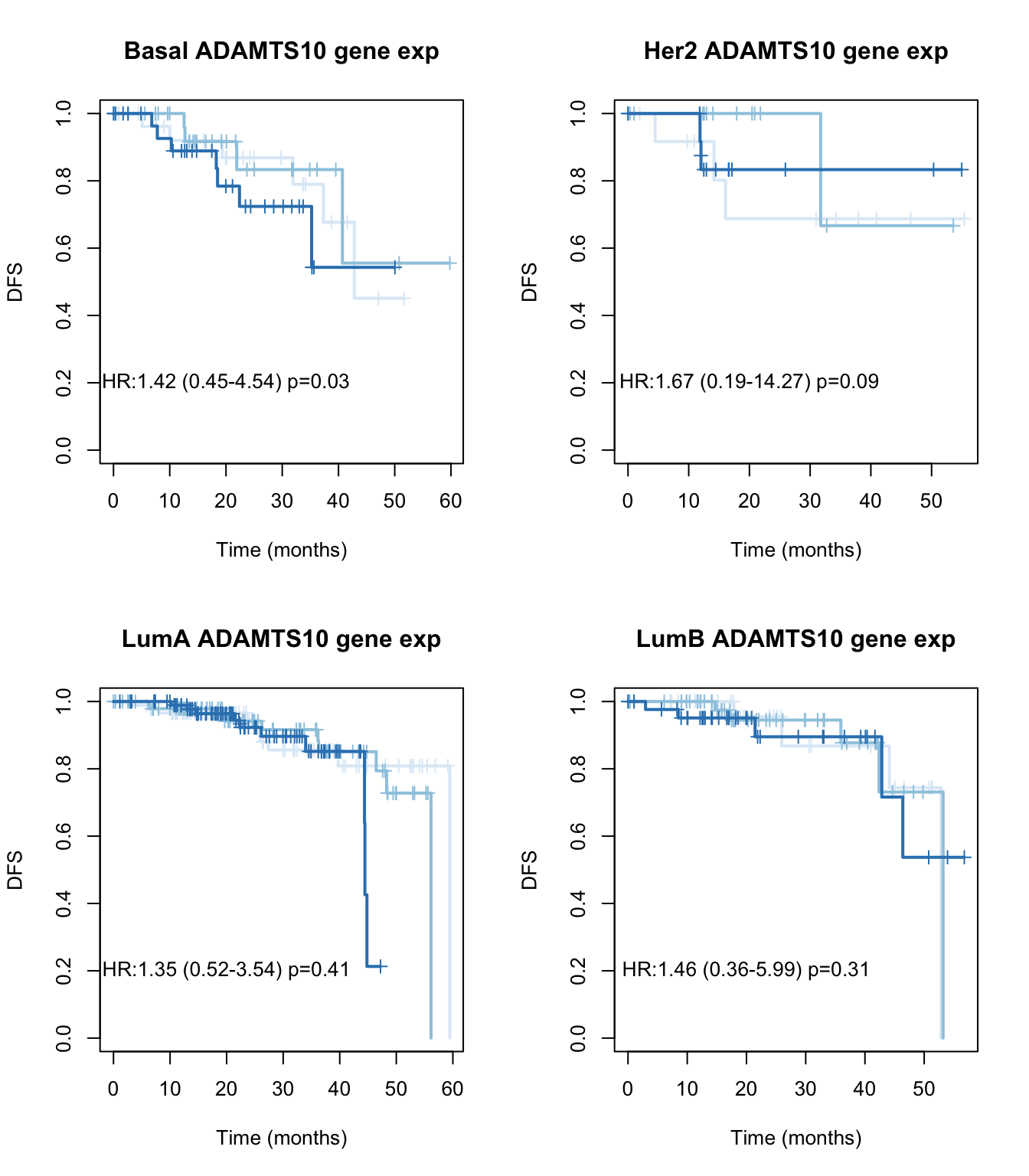
Figure 15.8: DFS ADAMTS10 by subtype
15.2.2 Redone using only ER cases
Redo survival and limit only to ER+ cases:
## make a change here
tinfoER=tinfo[which(tinfo$pam%in%c("LumA", "LumB")),  ]
tinfoER$pam=factor(tinfoER$pam)

axD=Surv(tinfoER$DFM, ifelse(tinfoER$DFS=="Recurred/Progressed", 1, ifelse(tinfoER$DFS=="DiseaseFree", 0, NA)))

axO=Surv(tinfoER$OSM, ifelse(tinfoER$OSS=="DECEASED", 1, ifelse(tinfoER$OSS=="LIVING", 0, NA)))

SurvOSS=coxph(axO~tinfoER$pam+tinfoER$Stage+tinfoER$adamts10)
SurvDFS=coxph(axD~tinfoER$pam+tinfoER$Stage+tinfoER$adamts10)

ao=summary(SurvOSS)
ao
## Call:
## coxph(formula = axO ~ tinfoER$pam + tinfoER$Stage + tinfoER$adamts10)
##
##   n= 580, number of events= 45
##    (2 observations deleted due to missingness)
##
##                     coef exp(coef) se(coef)     z Pr(>|z|)
## tinfoER$pamLumB   0.7352    2.0859   0.3289 2.235  0.02538 *
## tinfoER$Stage2    1.2321    3.4283   0.4604 2.676  0.00745 **
## tinfoER$Stage3    0.4820    1.6193   0.6456 0.747  0.45530
## tinfoER$Stage4    2.6492   14.1425   0.5702 4.646 3.39e-06 ***
## tinfoER$adamts10  0.3179    1.3742   0.1796 1.770  0.07672 .
## ---
## Signif. codes:  0 '***' 0.001 '**' 0.01 '*' 0.05 '.' 0.1 ' ' 1
##
##                  exp(coef) exp(-coef) lower .95 upper .95
## tinfoER$pamLumB      2.086    0.47942    1.0948     3.974
## tinfoER$Stage2       3.428    0.29169    1.3905     8.452
## tinfoER$Stage3       1.619    0.61754    0.4569     5.739
## tinfoER$Stage4      14.143    0.07071    4.6253    43.243
## tinfoER$adamts10     1.374    0.72769    0.9665     1.954
##
## Concordance= 0.682  (se = 0.044 )
## Likelihood ratio test= 27.23  on 5 df,   p=5e-05
## Wald test            = 28.36  on 5 df,   p=3e-05
## Score (logrank) test = 35.76  on 5 df,   p=1e-06
as=summary(SurvDFS)
as
## Call:
## coxph(formula = axD ~ tinfoER$pam + tinfoER$Stage + tinfoER$adamts10)
##
##   n= 431, number of events= 44
##    (151 observations deleted due to missingness)
##
##                    coef exp(coef) se(coef)     z Pr(>|z|)
## tinfoER$pamLumB  0.3624    1.4367   0.3493 1.038  0.29949
## tinfoER$Stage2   0.6869    1.9875   0.4159 1.651  0.09866 .
## tinfoER$Stage3   1.1168    3.0550   0.5321 2.099  0.03583 *
## tinfoER$Stage4   1.8789    6.5462   0.6964 2.698  0.00698 **
## tinfoER$adamts10 0.3702    1.4480   0.1702 2.175  0.02966 *
## ---
## Signif. codes:  0 '***' 0.001 '**' 0.01 '*' 0.05 '.' 0.1 ' ' 1
##
##                  exp(coef) exp(-coef) lower .95 upper .95
## tinfoER$pamLumB      1.437     0.6960    0.7246     2.849
## tinfoER$Stage2       1.987     0.5032    0.8795     4.491
## tinfoER$Stage3       3.055     0.3273    1.0767     8.668
## tinfoER$Stage4       6.546     0.1528    1.6718    25.633
## tinfoER$adamts10     1.448     0.6906    1.0372     2.022
##
## Concordance= 0.588  (se = 0.052 )
## Likelihood ratio test= 12.76  on 5 df,   p=0.03
## Wald test            = 13.76  on 5 df,   p=0.02
## Score (logrank) test = 14.92  on 5 df,   p=0.01
#pdf("figure-outputs/NEwpanelB.pdf", height=7, width=9)
par(mfrow=c(2,3))
boxplot(tinfoER$adamts10~tinfoER$pam, ylab="gene exp", main="PAM50")
boxplot(tinfoER$adamts10~tinfoER$immSub, ylab="gene exp", main="Immune sbtype")
ax=cor.test(tinfoER$adamts10, log10(tinfoER$codingMut+1), method="spearman")
smoothScatter(tinfoER$adamts10, log10(tinfoER$codingMut+1), xlab="gene exp", ylab="log10 mut")
text(4,0.5, sprintf("cor=%s, p=%s", round(ax$estimate, 2), round(ax$p.value, 3)))
ax=cor.test(tinfoER$adamts10, tinfoER$leukFrac, method="spearman")
smoothScatter(tinfoER$adamts10, (tinfoER$leukFrac), xlab="gene exp", ylab="leuk frac")
text(4,0.2, sprintf("cor=%s, p=%s", round(ax$estimate, 2), round(ax$p.value, 3)))
ax=cor.test(tinfoER$adamts10, tinfoER$TCRshann, method="spearman")
smoothScatter(tinfoER$adamts10, tinfoER$TCRshann, xlab="gene exp", ylab="TCR diversity")
text(4,1, sprintf("cor=%s, p=%s", round(ax$estimate, 2), round(ax$p.value, 3)))
ax=cor.test(tinfoER$adamts10, tinfoER$strFrac, method="spearman")
smoothScatter(tinfoER$adamts10, (tinfoER$strFrac), xlab="gene exp", ylab="str frac")
text(4,0.2, sprintf("cor=%s, p=%s", round(ax$estimate, 2), round(ax$p.value, 3)))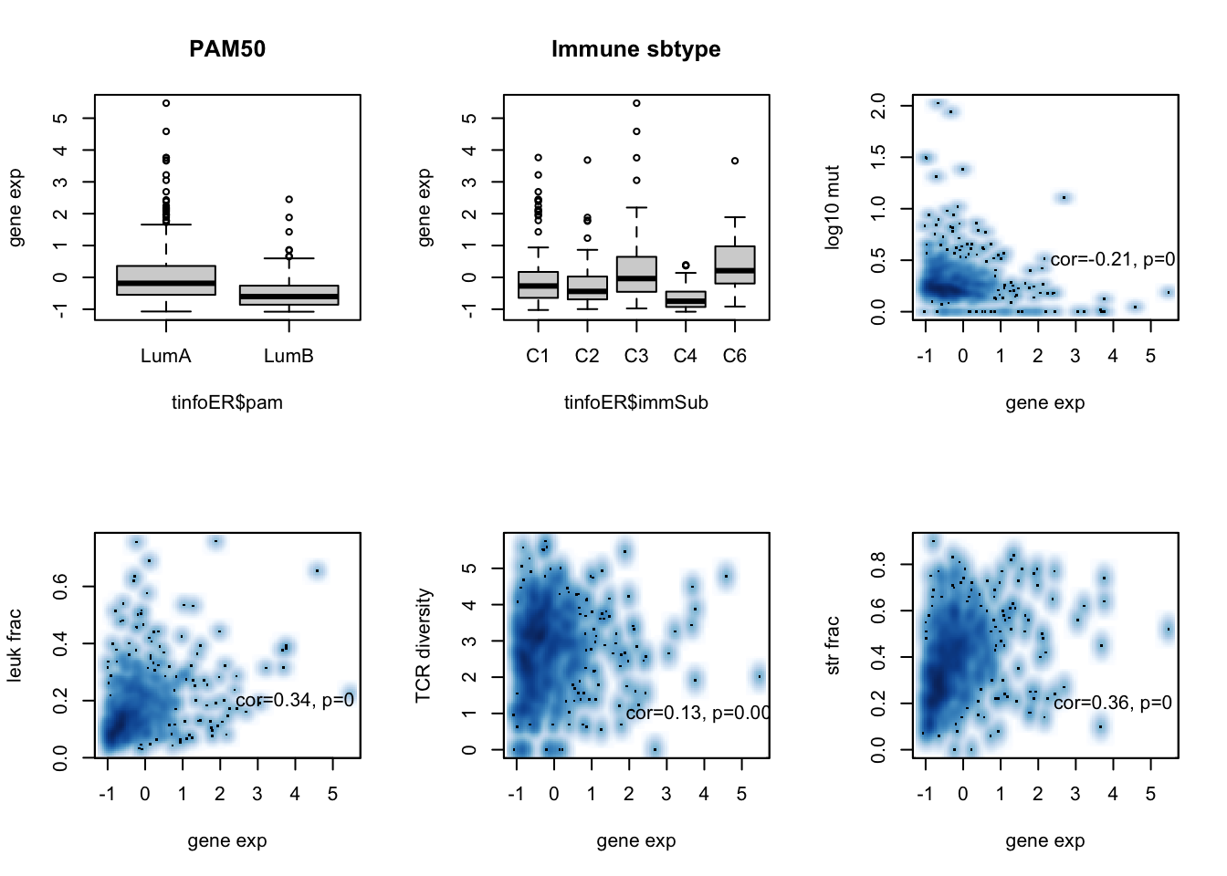
DT::datatable(tinfoER, rownames=F, class='cell-border stripe',
          extensions="Buttons", options=list(dom="Bfrtip", buttons=c('csv', 'excel')))
Also check the forest plots
data1=data.frame(X1=c("","PAM50", "",  "Stage", "","","", "ADAMST10"),
                X2=c("","LumA", "LumB" ,"1", "2", "3", "4", ""),
                X3=c("NSamp",  table(tinfoER$pam), table(tinfoER$Stage), length(na.omit(tinfoER$adamts10))),
                X4=c("HR", "", round(summary(SurvOSS)$coefficients[ 1,2],2), "",
                     round(summary(SurvOSS)$coefficients[ 2:5,2],2)))

mdata=data.frame(summary(SurvOSS)$conf.int[ ,c(1,3:4)])
mdata=rbind(NA,NA, mdata[1, ], NA, mdata[2:5, ])

#pdf("figure-outputs/Figure5_CD74_forestplot.pdf", width=5, height=5)

forestplot(data1, mdata, xlog=T,
           boxsize=0.5)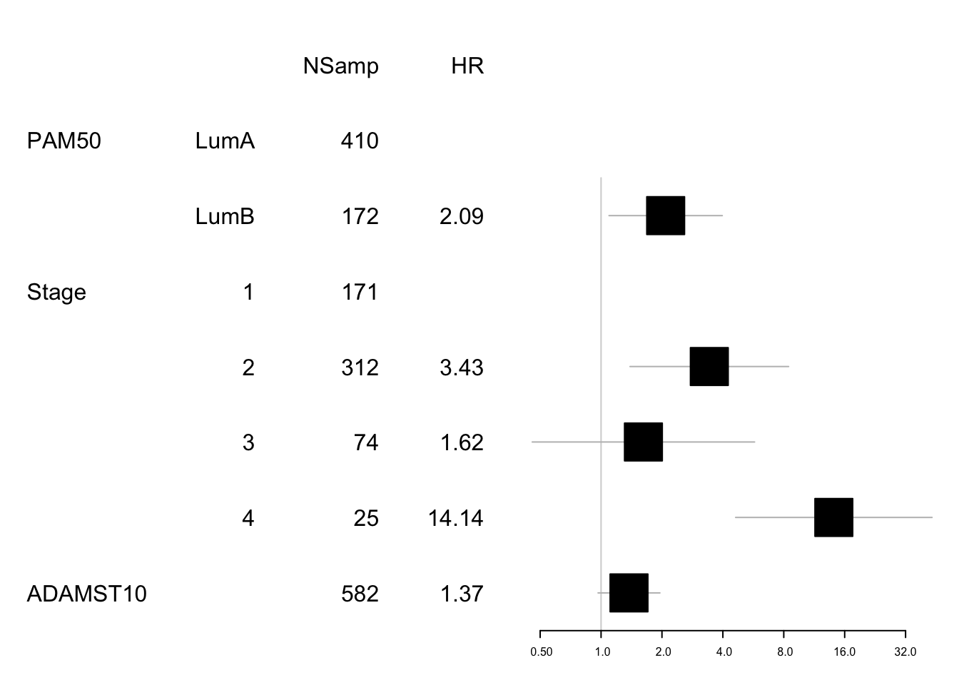
Figure 15.9: Adamts10 expression survival analysis, ER only
DT::datatable(cbind(data1, mdata), rownames=F, class='cell-border stripe',
          extensions="Buttons", options=list(dom="Bfrtip", buttons=c('csv', 'excel')))
Figure 15.9: Adamts10 expression survival analysis, ER only
15.3 Signature: Lum cases non-inflammatory: growing vs stable
Here, use the signature which was applied before to see the difference between the non-inflammatory growing vs stable samples. We compare this to the oncotypedx list of genes and mammaprint
#GlistGrowing=rownames(vstLumRes)[which(vstLumRes$log2FoldChange>1.5 & vstLumRes$baseMean>100 & vstLumRes$padj<0.05 )]
#Glistnon=rownames(vstLumRes)[which(vstLumRes$log2FoldChange<(-1.5) & vstLumRes$baseMean>100 & vstLumRes$padj<0.05 )]

HumGeneList=SymHum2Rat$HGNC.symbol[match(GlistGrowing, SymHum2Rat$RGD.symbol)]
HumGeneList2=Rat2Hum$HGNC.symbol[match(GlistGrowing, Rat2Hum$RGD.symbol)]

TCGAssgsea=gsva((TCGArsem2), list(grow=na.omit(HumGeneList2),
                                                stab=Rat2Hum$HGNC.symbol[match(Glistnon, Rat2Hum$RGD.symbol)], Onco=Oncoprint[[1]], Mamma=Oncoprint[[2]]), method="ssgsea", ssgsea.norm=F)

TCGAssgsea=t(scale(t(TCGAssgsea)))

par(mfrow=c(1,2))
hist(TCGAssgsea[1, ], main="stable")
hist(TCGAssgsea[2, ], main="growing")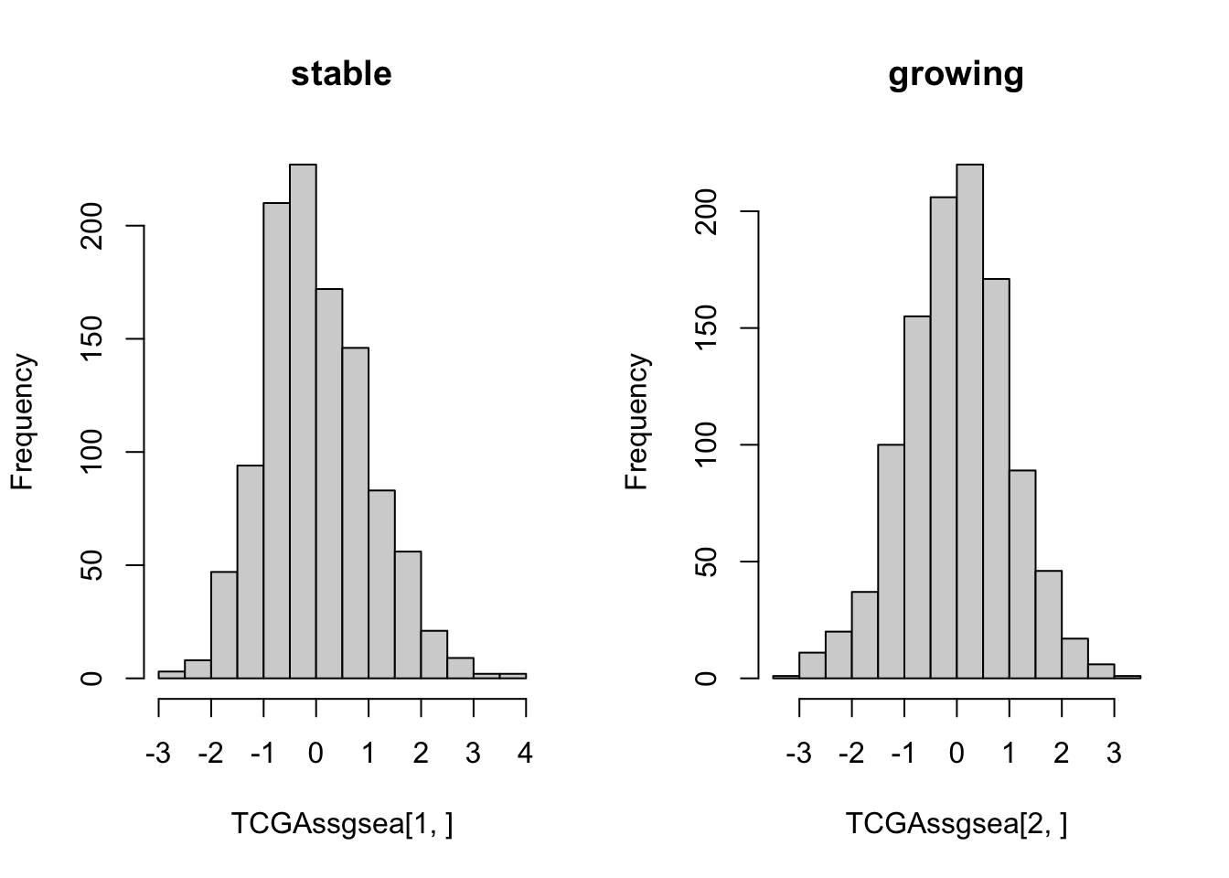
plot(TCGAssgsea[1, ], TCGAssgsea[2, ], xlab="stable", ylab="growing")

## also compare with onco or mamma print

plot(TCGAssgsea[1, ], TCGAssgsea[3, ], xlab="stable", ylab="oncotype")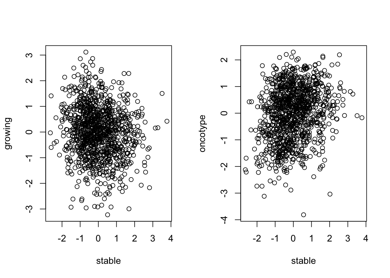
plot(TCGAssgsea[1, ], TCGAssgsea[4, ], xlab="stable", ylab="mammaprint")


write.csv("nature-tables/Supplemental_table5.csv")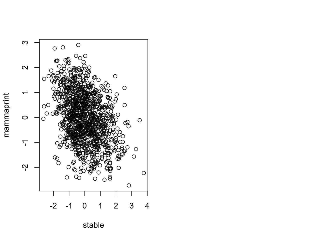
The Growing signature genes (positive coefficient) are Setd7, Hspa1l, Hbb, Kifc2, Kmt5c, Pik3c2b, Lmntd2, Nsmf, Nrbp2, LOC100134871, Hsp90aa1, Coro6, Chst8, Slc4a3, Fhod1, Rpl8, Spp1, Catsperg, Col5a1, LOC100911498, Noxa1, F8, Rps19, Rps6, Irs1, Leng8, Plekhh1, Lmbr1l, Ikbke, Pnisr, Adamts10, Zfp692, Trim41, Sema6d, Mgp, Cdc42bpg, Slc16a13, Dmpk and stable (negative coefficient) are Fgfr2, Mx1, Endou, Grhl3, Slpi, Gbp2, Plg, Aldh1a3, Upk3a.
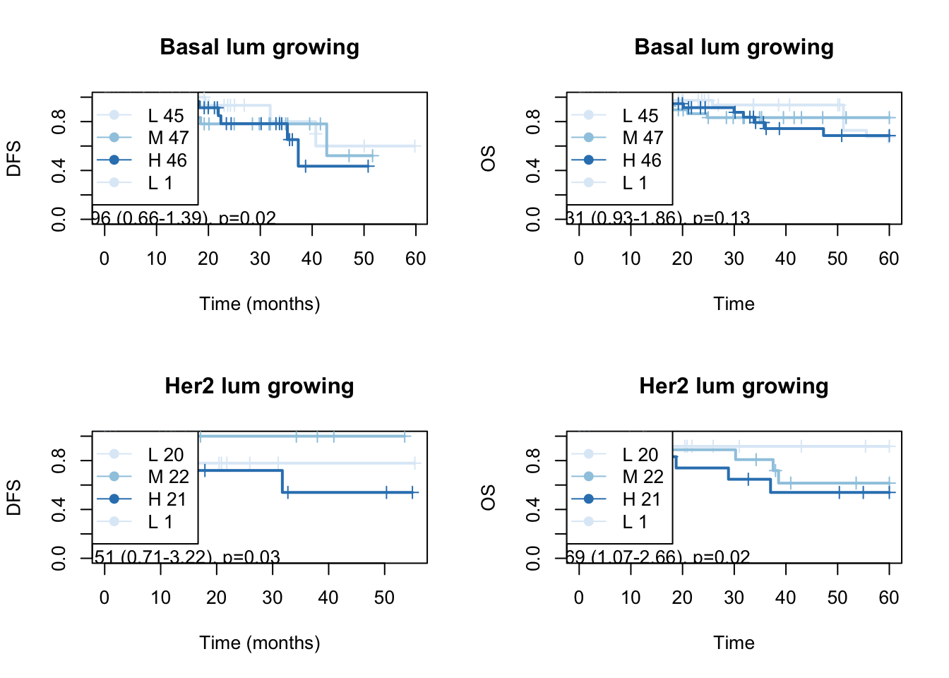
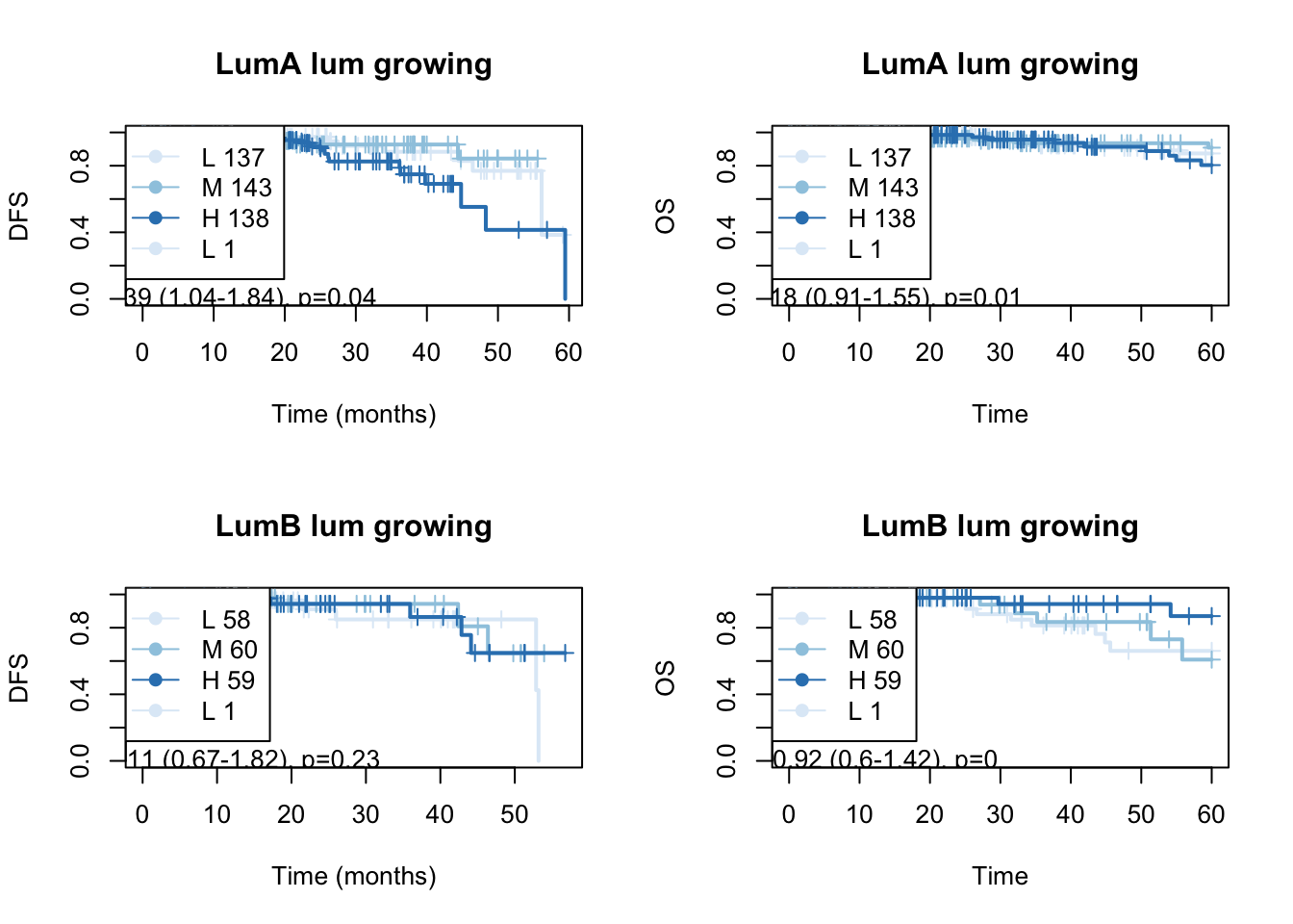
Below are the survival curves for the growing signature:
#pdf("figure-outputs/Fig5_survival_analysis__poslist_Lum_samples_baseMean_greater100.pdf", height=8, width = 8)

par(mfrow=c(2,2))

Xind=c("Basal", "Her2", "LumA", "LumB")

for (i in Xind){
  l1=which(BrClin$PAM50==i)
  lx2=match(BrClin$Patient.ID[l1], colnames(TCGArsem2))
  ax=Surv(BrClin$Overall.Survival..Months.[l1], ifelse(BrClin$Overall.Survival.Status[l1]=="DECEASED", 1, ifelse(BrClin$Overall.Survival.Status[l1]=="LIVING", 0, NA)))
   axb=coxph(ax~TCGAssgsea[1, lx2]+BrClin$Stage[l1])
  axc=summary(axb)
  TCGAvalCut=cut(TCGAssgsea[1, lx2], quantile(TCGAssgsea[1, lx2], c(0, 0.33, 0.67, 1)), c("L","M", "P"))
  ax2=plot(survfit(ax~TCGAvalCut), main=paste(i, "lum growing"), col=brewer.pal(3, "Blues"),lwd=2, xlab="Time (months)", ylab="OS", mark.time=T)
   text(10, 0, sprintf("univ. cts. var. HR=%s (%s-%s), p=%s", round(axc$coefficients[1,2], 2),
                      round(axc$conf.int[1,3],2), round(axc$conf.int[1,4],2),round(axc$logtest[3],2 )))
   legend("topleft",paste(c("L", "M", "H"), summary(TCGAvalCut)), col=brewer.pal(3, "Blues"), lwd=1,
          pch=19)

}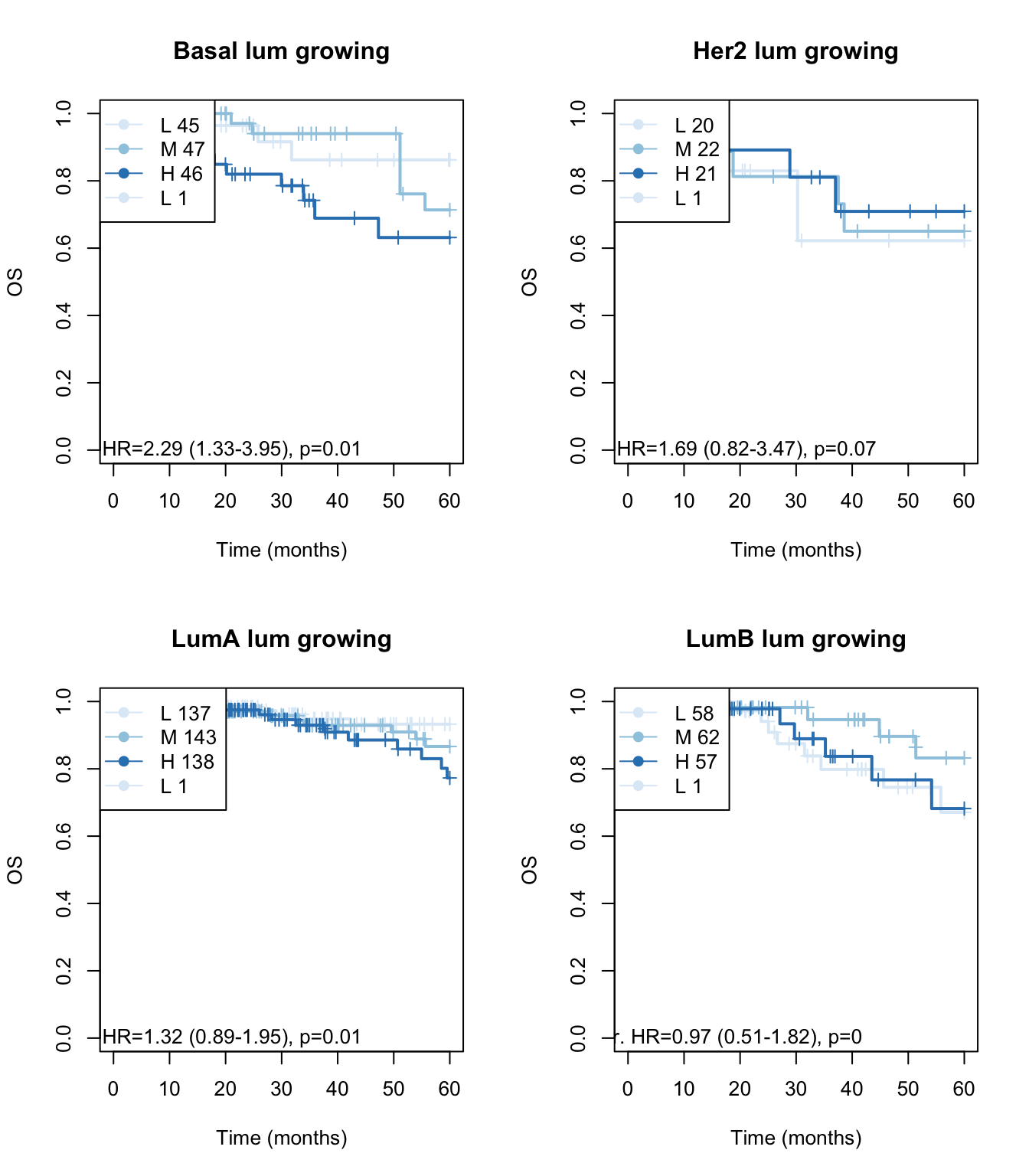
Figure 15.10: OS: growing signature
for (i in Xind){
  l1=which(BrClin$PAM50==i)
  lx2=match(BrClin$Patient.ID[l1], colnames(TCGArsem2))
  ax=Surv(BrClin$Disease.Free..Months.[l1], ifelse(BrClin$Disease.Free.Status[l1]=="Recurred/Progressed", 1, ifelse(BrClin$Disease.Free.Status[l1]=="DiseaseFree", 0, NA)))
  axb=coxph(ax~TCGAssgsea[1, lx2]+BrClin$Stage[l1])
  axc=summary(axb)

  TCGAvalCut=cut(TCGAssgsea[1, lx2], quantile(TCGAssgsea[1, lx2], c(0, 0.33, 0.67, 1)), c("L","M", "P"))
  ax2=plot(survfit(ax~TCGAvalCut), main=paste(i, "lum growing"), col=brewer.pal(3, "Blues"),lwd=2, xlab="Time (months)", ylab="DFS", mark.time=T)
  text(10, 0, sprintf("univ. cts. var. HR=%s (%s-%s), p=%s", round(axc$coefficients[1,2], 2),
                      round(axc$conf.int[1,3],2), round(axc$conf.int[1,4],2),round(axc$logtest[3],2 )))
 legend("topleft",paste(c("L", "M", "H"), summary(TCGAvalCut)), col=brewer.pal(3, "Blues"), lwd=1,
          pch=19)
}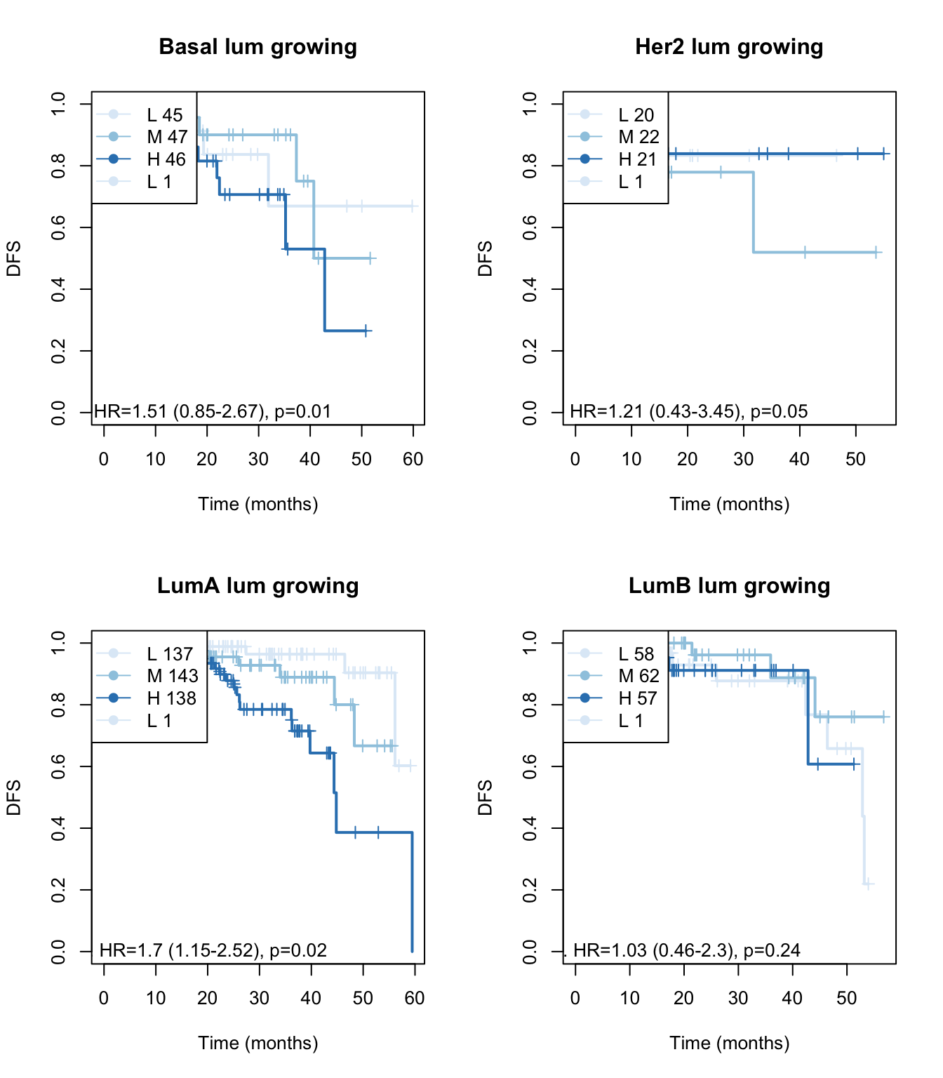
Figure 15.11: OS: growing signature
#dev.off()

#DT::datatable(as.data.frame(test), rownames=F, class='cell-border stripe',
#         extensions="Buttons", options=list(dom="Bfrtip", buttons=c('csv', 'excel')))
The OS curves for the stable signature
#pdf("figure-outputs/Fig5_survival_analysis__neglist_Lum_samples_baseMean_greater100.pdf", height=8, width = 8)

par(mfrow=c(2,2))

Xind=c("Basal", "Her2", "LumA", "LumB")

for (i in Xind){
  l1=which(BrClin$PAM50==i)
   lx2=match(BrClin$Patient.ID[l1], colnames(TCGArsem2))
  ax=Surv(BrClin$Overall.Survival..Months.[l1], ifelse(BrClin$Overall.Survival.Status[l1]=="DECEASED", 1, ifelse(BrClin$Overall.Survival.Status[l1]=="LIVING", 0, NA)))
   axb=coxph(ax~TCGAssgsea[2, lx2]+BrClin$Stage[l1])
  axc=summary(axb)

  TCGAvalCut=cut(TCGAssgsea[2, lx2], quantile(TCGAssgsea[2, lx2], c(0, 0.33, 0.67, 1)), c("L","M", "P"))
  ax2=plot(survfit(ax~TCGAvalCut), main=paste(i, "lum stab"), col=brewer.pal(3, "Blues"),lwd=2, xlab="Time", ylab="OS", mark.time=T)
   text(10, 0, sprintf("univ. cts. var. HR=%s (%s-%s), p=%s", round(axc$coefficients[1,2], 2),
                      round(axc$conf.int[1,3],2), round(axc$conf.int[1,4],2),round(axc$logtest[3],2 )))
 #  legend("topleft",paste(c("L", "M", "H"), summary(TCGAvalCut)), col=brewer.pal(3, "Blues"), lwd=1,
#          pch=19)

}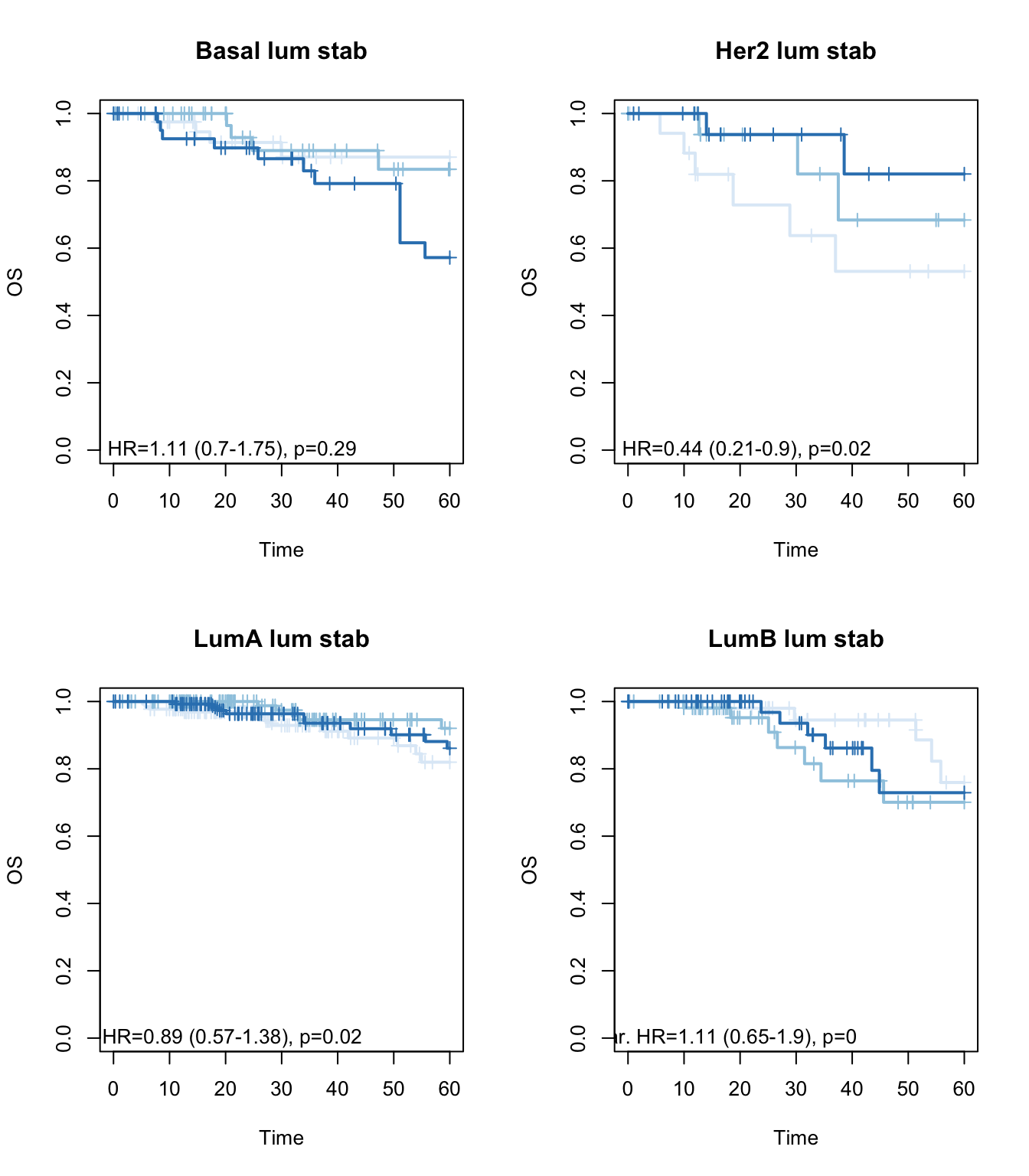
Figure 15.12: OS: stable signature
#dev.off()

ax=cut(TCGAssgsea[2, lx2], quantile(TCGAssgsea[2, lx2], c(0, 0.33, 0.67, 1)), c("L","M", "P"))
table(ax)
## ax
##  L  M  P
## 58 60 59

par(mfrow=c(2,2))

for (i in Xind){
  l1=which(BrClin$PAM50==i)
   lx2=match(BrClin$Patient.ID[l1], colnames(TCGArsem2))
  ax=Surv(BrClin$Disease.Free..Months.[l1], ifelse(BrClin$Disease.Free.Status[l1]=="Recurred/Progressed", 1, ifelse(BrClin$Disease.Free.Status[l1]=="DiseaseFree", 0, NA)))
   axb=coxph(ax~TCGAssgsea[2, lx2]+BrClin$Stage[l1])

  axc=summary(axb)
  axc
  TCGAvalCut=cut(TCGAssgsea[2, lx2], quantile(TCGAssgsea[2, lx2], c(0, 0.33, 0.67, 1)), c("L","M", "P"))
  ax2=plot(survfit(ax~TCGAvalCut), main=paste(i, "lum stable"), col=brewer.pal(3, "Blues"),lwd=2, xlab="Time (months)", ylab="DFS", mark.time=T)
    text(10, 0, sprintf("univ. cts. var. HR=%s (%s-%s), p=%s", round(axc$coefficients[1,2], 2),
                      round(axc$conf.int[1,3],2), round(axc$conf.int[1,4],2),round(axc$logtest[3],2 )))
#    legend("topleft",paste(c("L", "M", "H"), summary(TCGAvalCut)), col=brewer.pal(3, "Blues"), lwd=1,
#          pch=19)

}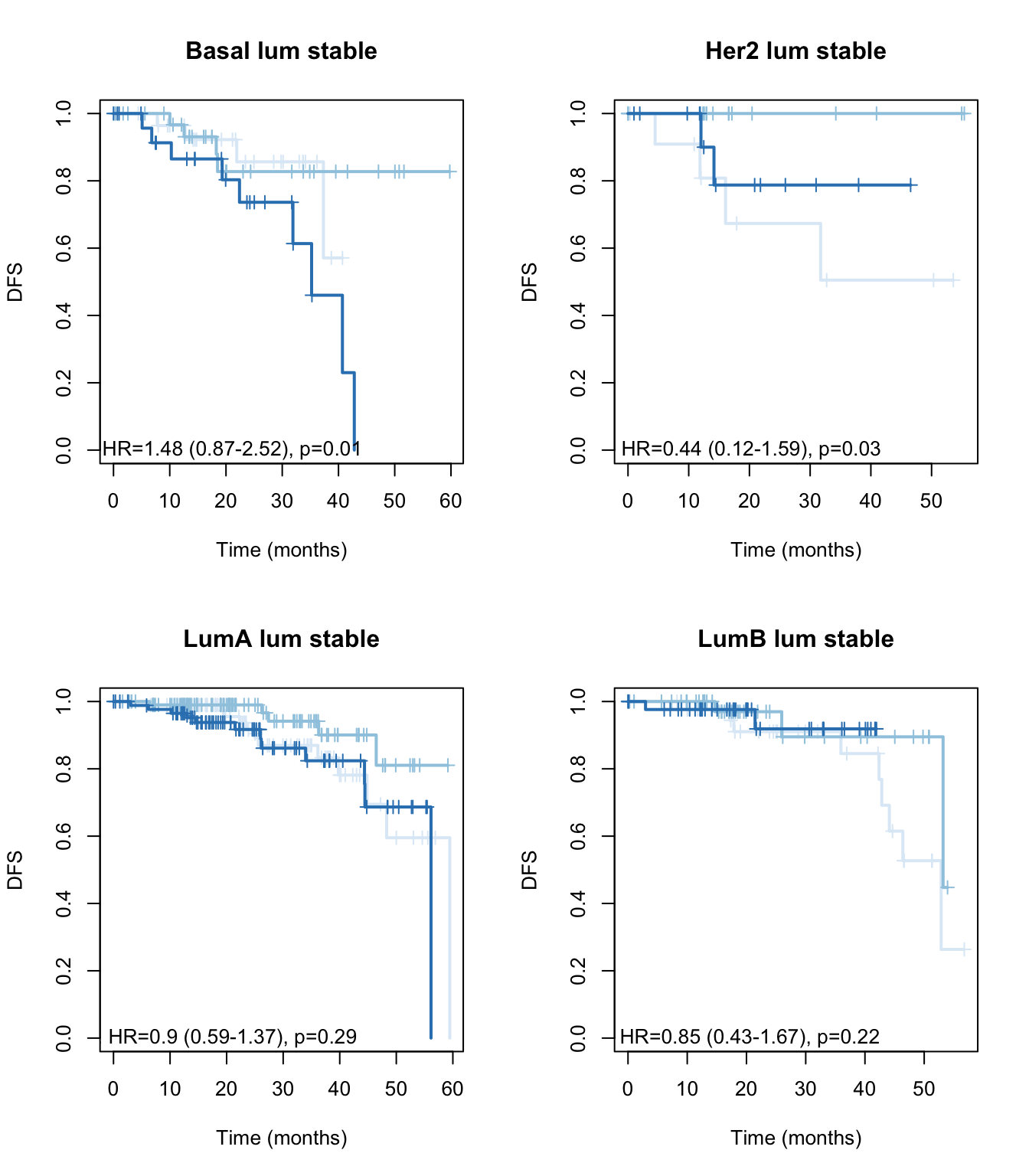
Figure 15.13: OS: stable signature
Quick sanity checks: for LuminalA samples, check that the scores match with outcome
## coxph for growing signature:
 l1=which(BrClin$PAM50=="LumA")
   lx2=match(BrClin$Patient.ID[l1], colnames(TCGAssgsea))
  ax=Surv(BrClin$Disease.Free..Months.[l1], ifelse(BrClin$Disease.Free.Status[l1]=="Recurred/Progressed", 1, ifelse(BrClin$Disease.Free.Status[l1]=="DiseaseFree", 0, NA)))
   axb=coxph(ax~TCGAssgsea[1, lx2]+BrClin$Stage[l1])
   summary(axb)
## Call:
## coxph(formula = ax ~ TCGAssgsea[1, lx2] + BrClin$Stage[l1])
##
##   n= 297, number of events= 30
##    (122 observations deleted due to missingness)
##
##                      coef exp(coef) se(coef)     z Pr(>|z|)
## TCGAssgsea[1, lx2] 0.5325    1.7032   0.2003 2.658  0.00786 **
## BrClin$Stage[l1]2  0.1482    1.1598   0.4742 0.313  0.75465
## BrClin$Stage[l1]3  0.7633    2.1455   0.5768 1.323  0.18570
## BrClin$Stage[l1]4  1.1378    3.1200   0.8184 1.390  0.16445
## ---
## Signif. codes:  0 '***' 0.001 '**' 0.01 '*' 0.05 '.' 0.1 ' ' 1
##
##                    exp(coef) exp(-coef) lower .95 upper .95
## TCGAssgsea[1, lx2]     1.703     0.5871    1.1501     2.522
## BrClin$Stage[l1]2      1.160     0.8622    0.4578     2.938
## BrClin$Stage[l1]3      2.145     0.4661    0.6927     6.645
## BrClin$Stage[l1]4      3.120     0.3205    0.6273    15.517
##
## Concordance= 0.678  (se = 0.045 )
## Likelihood ratio test= 11.87  on 4 df,   p=0.02
## Wald test            = 12.45  on 4 df,   p=0.01
## Score (logrank) test = 13.21  on 4 df,   p=0.01

## boxplot of growing signature with outcome:
par(mfrow=c(1,2))
boxplot(TCGAssgsea[1, lx2]~BrClin$Disease.Free.Status[l1], main="growing sig with status")
boxplot(TCGAssgsea[1, lx2]~BrClin$Overall.Survival.Status[l1], main="growing sig with OS") 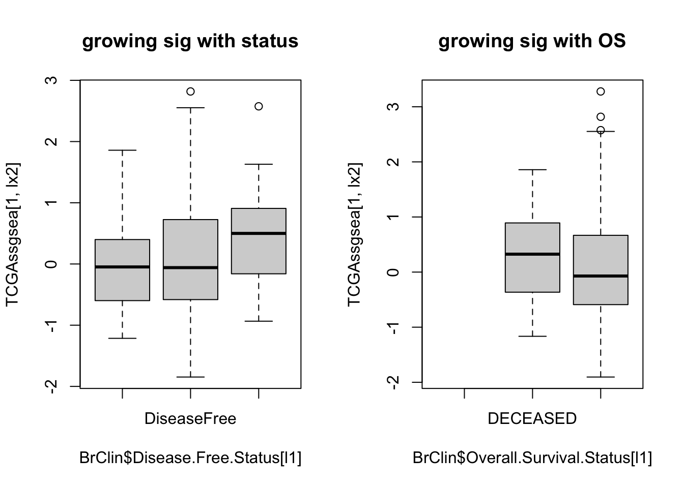
Combined signature: subtract the stable signature from the growing signature and check the outcome here:
#pdf("figure-outputs/Fig5_survival_analysis_growing_subtract_stab_Lum_samples_baseMean_greater100.pdf", height=8, width = 8)

par(mfrow=c(2,2))

for (i in Xind){
  l1=which(BrClin$PAM50==i)
   lx2=match(BrClin$Patient.ID[l1], colnames(TCGArsem2))
  ax=Surv(BrClin$Disease.Free..Months.[l1], ifelse(BrClin$Disease.Free.Status[l1]=="Recurred/Progressed", 1, ifelse(BrClin$Disease.Free.Status[l1]=="DiseaseFree", 0, NA)))
  tval=TCGAssgsea[1, lx2]-TCGAssgsea[2, lx2]
   axb=coxph(ax~tval+BrClin$Stage[l1])
  axc=summary(axb)
  TCGAvalCut=cut(tval, quantile(tval, c(0, 0.33, 0.67, 1)), c("L","M", "P"))
  ax2=plot(survfit(ax~TCGAvalCut), main=paste(i, "lum growing"), col=brewer.pal(3, "Blues"),lwd=2, xlab="Time (months)", ylab="DFS", mark.time=T)
    text(10, 0, sprintf("HR=%s (%s-%s), p=%s", round(axc$coefficients[1,2], 2),
                      round(axc$conf.int[1,3],2), round(axc$conf.int[1,4],2),round(axc$logtest[3],2 )))
    legend("topleft",paste(c("L", "M", "H"), summary(TCGAvalCut)), col=brewer.pal(3, "Blues"), lwd=1,
          pch=19)

    ay=Surv(BrClin$Overall.Survival..Months.[l1], ifelse(BrClin$Overall.Survival.Status[l1]=="DECEASED", 1, ifelse(BrClin$Overall.Survival.Status[l1]=="LIVING", 0, NA)))
   ayb=coxph(ay~tval+BrClin$Stage[l1])
   ayc=summary(ayb)
    ax2=plot(survfit(ay~TCGAvalCut), main=paste(i, "lum growing"), col=brewer.pal(3, "Blues"),lwd=2, xlab="Time", ylab="OS", mark.time=T)
   text(10, 0, sprintf("HR=%s (%s-%s), p=%s", round(ayc$coefficients[1,2], 2),
                      round(ayc$conf.int[1,3],2), round(ayc$conf.int[1,4],2),round(ayc$logtest[3],2 )))
   legend("topleft",paste(c("L", "M", "H"), summary(TCGAvalCut)), col=brewer.pal(3, "Blues"), lwd=1,
          pch=19)

}
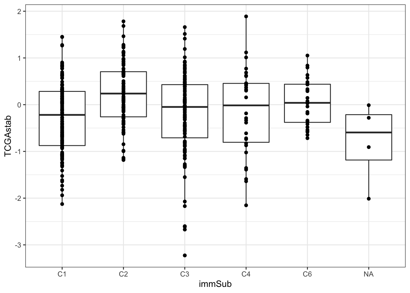
We can see whether this signature associates with leukocyte content and TCR diversity in the TCGA cohort:
l1=which(BrClin$PAM50=="LumA")
lx2=match(BrClin$Patient.ID[l1], colnames(TCGAssgsea))

lx3=match(BrClin$Patient.ID[l1], ThorssData$TCGA.Participant.Barcode)


newinfoTab=data.frame(pat=BrClin$Patient.ID[l1], TCGAgrow=TCGAssgsea[1, lx2],
                      TCGAstab=TCGAssgsea[2, lx2],
                      TCGAcomb=TCGAssgsea[1, lx2]-TCGAssgsea[2, lx2],
                      Onco=TCGAssgsea[3, lx2],
                      Mamma=TCGAssgsea[4, lx2],
                      OSM=BrClin$Overall.Survival..Months.[l1],
                      OSS=BrClin$Overall.Survival.Status[l1], DFS=BrClin$Disease.Free.Status[l1],
                 DFM=BrClin$Disease.Free..Months.[l1],
                 Stage=BrClin$Stage[l1],
                      leuk=as.numeric(ThorssData$Leukocyte.Fraction[lx3]),
                      str=as.numeric(ThorssData$Stromal.Fraction[lx3]),
                      TCRshann=as.numeric(ThorssData$TCR.Shannon[lx3]),
                      immSub=ThorssData$Immune.Subtype[lx3])


#pdf("figure-outputs/NewpanelC.pdf", height=8, width=9)
par(mfrow=c(2,2))
ax=cor.test(newinfoTab$TCGAgrow, newinfoTab$leuk, method="spearman")
smoothScatter(newinfoTab$TCGAgrow, newinfoTab$leuk,xlab="Luminal signature",
            ylab="Leukoycte")
text(0.6,0.6, sprintf("cor=%s, p=%s", round(ax$estimate, 2), round(ax$p.value, 2)))
ax=cor.test(newinfoTab$TCGAgrow, newinfoTab$str, method="spearman")
smoothScatter(newinfoTab$TCGAgrow, newinfoTab$str, xlab="Luminal signature",
            ylab="Stroma")
text(0.6,0.6, sprintf("cor=%s, p=%s", round(ax$estimate, 2), round(ax$p.value, 2)))
ax=cor.test(newinfoTab$TCGAgrow, newinfoTab$TCRshann, method="spearman")
smoothScatter(newinfoTab$TCGAgrow, newinfoTab$TCRshann,xlab="Luminal signature", ylab="TCR div")
text(0.6,5, sprintf("cor=%s, p=%s", round(ax$estimate, 2), round(ax$p.value, 9)))
boxplot(newinfoTab$TCGAgrow~newinfoTab$immSub)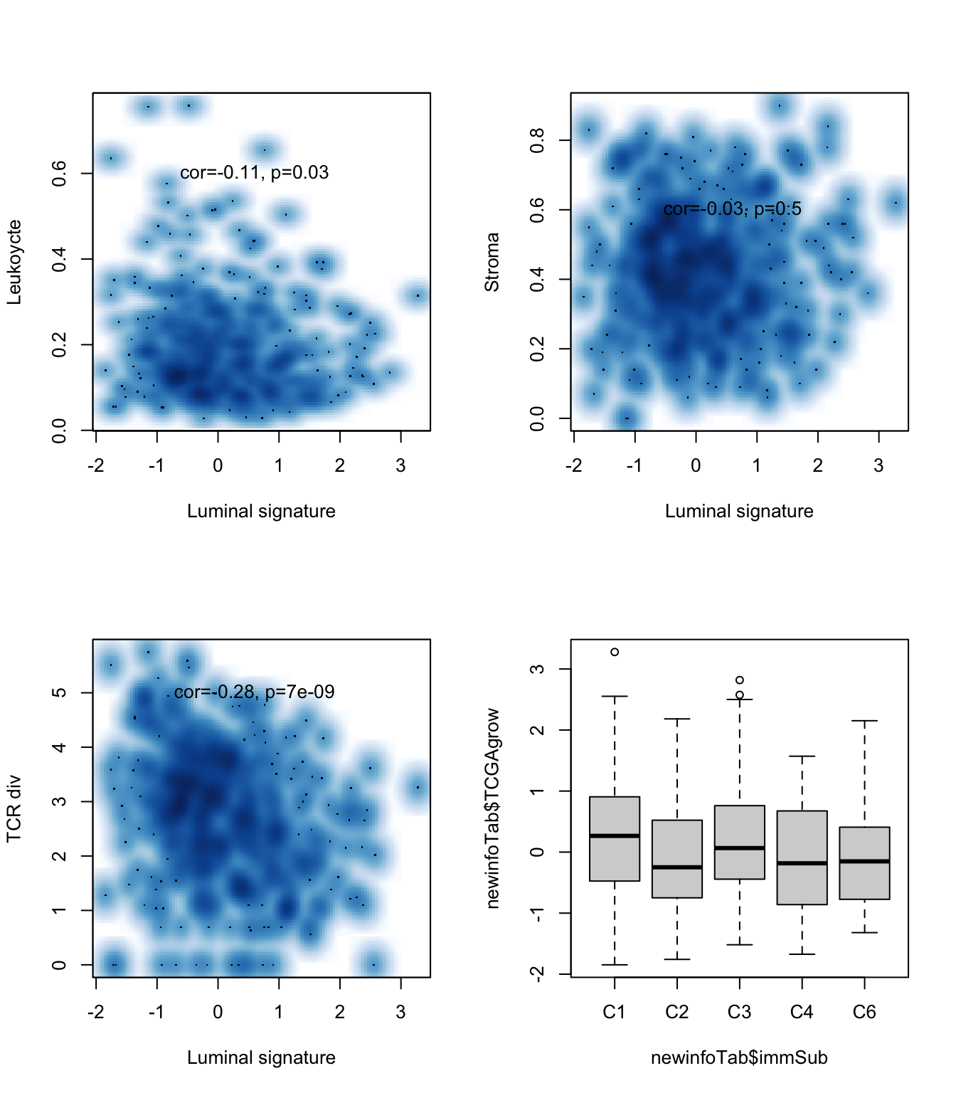
Figure 15.14: luminal signature associated with clinical variables
#dev.off()

DT::datatable(newinfoTab, rownames=T, class='cell-border stripe',
          extensions="Buttons", options=list(dom="Bfrtip", buttons=c('csv', 'excel'), Xscroll=T))
Figure 15.14: luminal signature associated with clinical variables
As well as whether it associates with any of the previously identified immune subtypes:
15.4 Comparison to oncotype and mammaprint
Finally, see how these compare to oncotype or mammaprint.
We can do this two ways:
15.4.1 Overall survival
- Run survival ~ Oncotype/Mamma/Growing + PAM50 + Stage
SurvOS=Surv(newinfoTab$OSM, ifelse(newinfoTab$OSS=="LIVING", 0, 1))
SurvDFS=Surv(newinfoTab$DFM, ifelse(newinfoTab$DFS=="DiseaseFree", 0,ifelse(newinfoTab$DFS=="Recurred/Progressed", 1, NA) ))

model1=coxph(SurvOS~TCGAgrow+Stage, data=newinfoTab)
summary(model1)
## Call:
## coxph(formula = SurvOS ~ TCGAgrow + Stage, data = newinfoTab)
##
##   n= 417, number of events= 27
##    (2 observations deleted due to missingness)
##
##             coef exp(coef) se(coef)      z Pr(>|z|)
## TCGAgrow  0.2753    1.3169   0.2012  1.368  0.17131
## Stage2    0.7334    2.0821   0.4799  1.528  0.12644
## Stage3   -0.9157    0.4003   1.0805 -0.847  0.39677
## Stage4    2.0093    7.4585   0.6467  3.107  0.00189 **
## ---
## Signif. codes:  0 '***' 0.001 '**' 0.01 '*' 0.05 '.' 0.1 ' ' 1
##
##          exp(coef) exp(-coef) lower .95 upper .95
## TCGAgrow    1.3169     0.7594   0.88770     1.954
## Stage2      2.0821     0.4803   0.81290     5.333
## Stage3      0.4003     2.4984   0.04815     3.327
## Stage4      7.4585     0.1341   2.09976    26.493
##
## Concordance= 0.667  (se = 0.058 )
## Likelihood ratio test= 13.72  on 4 df,   p=0.008
## Wald test            = 14.54  on 4 df,   p=0.006
## Score (logrank) test = 18.36  on 4 df,   p=0.001
model2=coxph(SurvOS~TCGAgrow+Onco+Stage, data=newinfoTab)
summary(model2)
## Call:
## coxph(formula = SurvOS ~ TCGAgrow + Onco + Stage, data = newinfoTab)
##
##   n= 417, number of events= 27
##    (2 observations deleted due to missingness)
##
##             coef exp(coef) se(coef)      z Pr(>|z|)
## TCGAgrow  0.3674    1.4440   0.2077  1.769  0.07694 .
## Onco     -0.6667    0.5134   0.2402 -2.776  0.00551 **
## Stage2    0.8442    2.3261   0.4839  1.744  0.08109 .
## Stage3   -0.9671    0.3802   1.0807 -0.895  0.37087
## Stage4    2.0347    7.6502   0.6615  3.076  0.00210 **
## ---
## Signif. codes:  0 '***' 0.001 '**' 0.01 '*' 0.05 '.' 0.1 ' ' 1
##
##          exp(coef) exp(-coef) lower .95 upper .95
## TCGAgrow    1.4440     0.6925   0.96106    2.1695
## Onco        0.5134     1.9478   0.32062    0.8221
## Stage2      2.3261     0.4299   0.90094    6.0055
## Stage3      0.3802     2.6303   0.04572    3.1617
## Stage4      7.6502     0.1307   2.09232   27.9719
##
## Concordance= 0.713  (se = 0.049 )
## Likelihood ratio test= 21.12  on 5 df,   p=8e-04
## Wald test            = 22.82  on 5 df,   p=4e-04
## Score (logrank) test = 26.15  on 5 df,   p=8e-05
model3=coxph(SurvOS~TCGAgrow+Mamma+Stage, data=newinfoTab)
summary(model3)
## Call:
## coxph(formula = SurvOS ~ TCGAgrow + Mamma + Stage, data = newinfoTab)
##
##   n= 417, number of events= 27
##    (2 observations deleted due to missingness)
##
##             coef exp(coef) se(coef)      z Pr(>|z|)
## TCGAgrow  0.2715    1.3119   0.2019  1.345  0.17878
## Mamma    -0.0464    0.9547   0.2459 -0.189  0.85035
## Stage2    0.7497    2.1164   0.4874  1.538  0.12401
## Stage3   -0.9201    0.3985   1.0809 -0.851  0.39463
## Stage4    2.0398    7.6894   0.6658  3.064  0.00219 **
## ---
## Signif. codes:  0 '***' 0.001 '**' 0.01 '*' 0.05 '.' 0.1 ' ' 1
##
##          exp(coef) exp(-coef) lower .95 upper .95
## TCGAgrow    1.3119     0.7622   0.88314     1.949
## Mamma       0.9547     1.0475   0.58954     1.546
## Stage2      2.1164     0.4725   0.81415     5.502
## Stage3      0.3985     2.5095   0.04791     3.315
## Stage4      7.6894     0.1300   2.08531    28.354
##
## Concordance= 0.664  (se = 0.058 )
## Likelihood ratio test= 13.76  on 5 df,   p=0.02
## Wald test            = 14.48  on 5 df,   p=0.01
## Score (logrank) test = 18.36  on 5 df,   p=0.003
modelos=coxph(SurvOS~TCGAgrow+Mamma+Onco+Stage, data=newinfoTab)
summary(modelos)
## Call:
## coxph(formula = SurvOS ~ TCGAgrow + Mamma + Onco + Stage, data = newinfoTab)
##
##   n= 417, number of events= 27
##    (2 observations deleted due to missingness)
##
##             coef exp(coef) se(coef)      z Pr(>|z|)
## TCGAgrow  0.4387    1.5507   0.2195  1.999  0.04565 *
## Mamma     0.3709    1.4491   0.2849  1.302  0.19290
## Onco     -0.8402    0.4316   0.2690 -3.123  0.00179 **
## Stage2    0.7444    2.1052   0.4932  1.509  0.13123
## Stage3   -0.9419    0.3899   1.0810 -0.871  0.38361
## Stage4    1.8090    6.1043   0.6920  2.614  0.00895 **
## ---
## Signif. codes:  0 '***' 0.001 '**' 0.01 '*' 0.05 '.' 0.1 ' ' 1
##
##          exp(coef) exp(-coef) lower .95 upper .95
## TCGAgrow    1.5507     0.6449   1.00851    2.3845
## Mamma       1.4491     0.6901   0.82908    2.5328
## Onco        0.4316     2.3168   0.25476    0.7313
## Stage2      2.1052     0.4750   0.80068    5.5351
## Stage3      0.3899     2.5647   0.04686    3.2443
## Stage4      6.1043     0.1638   1.57250   23.6964
##
## Concordance= 0.742  (se = 0.044 )
## Likelihood ratio test= 22.88  on 6 df,   p=8e-04
## Wald test            = 25.63  on 6 df,   p=3e-04
## Score (logrank) test = 28.26 on 6 df, p=8e-05- Also try the stable signature:
model1=coxph(SurvOS~TCGAstab+Stage, data=newinfoTab)
summary(model1)
## Call:
## coxph(formula = SurvOS ~ TCGAstab + Stage, data = newinfoTab)
##
##   n= 417, number of events= 27
##    (2 observations deleted due to missingness)
##
##             coef exp(coef) se(coef)      z Pr(>|z|)
## TCGAstab -0.1176    0.8890   0.2232 -0.527  0.59818
## Stage2    0.7431    2.1025   0.4796  1.549  0.12128
## Stage3   -0.8446    0.4297   1.0810 -0.781  0.43461
## Stage4    2.0023    7.4064   0.6553  3.055  0.00225 **
## ---
## Signif. codes:  0 '***' 0.001 '**' 0.01 '*' 0.05 '.' 0.1 ' ' 1
##
##          exp(coef) exp(-coef) lower .95 upper .95
## TCGAstab    0.8890     1.1248   0.57400     1.377
## Stage2      2.1025     0.4756   0.82127     5.382
## Stage3      0.4297     2.3271   0.05165     3.575
## Stage4      7.4064     0.1350   2.05019    26.756
##
## Concordance= 0.67  (se = 0.063 )
## Likelihood ratio test= 12.19  on 4 df,   p=0.02
## Wald test            = 13.06  on 4 df,   p=0.01
## Score (logrank) test = 16.83  on 4 df,   p=0.002
model2=coxph(SurvOS~TCGAstab+Onco+Stage, data=newinfoTab)
summary(model2)
## Call:
## coxph(formula = SurvOS ~ TCGAstab + Onco + Stage, data = newinfoTab)
##
##   n= 417, number of events= 27
##    (2 observations deleted due to missingness)
##
##             coef exp(coef) se(coef)      z Pr(>|z|)
## TCGAstab -0.2364    0.7895   0.2126 -1.112  0.26621
## Onco     -0.6851    0.5040   0.2530 -2.708  0.00677 **
## Stage2    0.8198    2.2700   0.4817  1.702  0.08879 .
## Stage3   -0.8871    0.4118   1.0815 -0.820  0.41206
## Stage4    1.8823    6.5685   0.6615  2.845  0.00443 **
## ---
## Signif. codes:  0 '***' 0.001 '**' 0.01 '*' 0.05 '.' 0.1 ' ' 1
##
##          exp(coef) exp(-coef) lower .95 upper .95
## TCGAstab    0.7895     1.2667   0.52039    1.1976
## Onco        0.5040     1.9840   0.30697    0.8276
## Stage2      2.2700     0.4405   0.88307    5.8353
## Stage3      0.4118     2.4281   0.04945    3.4300
## Stage4      6.5685     0.1522   1.79635   24.0184
##
## Concordance= 0.703  (se = 0.055 )
## Likelihood ratio test= 19.3  on 5 df,   p=0.002
## Wald test            = 21.8  on 5 df,   p=6e-04
## Score (logrank) test = 24.82  on 5 df,   p=2e-04
model3=coxph(SurvOS~TCGAstab+Mamma+Stage, data=newinfoTab)
summary(model3)
## Call:
## coxph(formula = SurvOS ~ TCGAstab + Mamma + Stage, data = newinfoTab)
##
##   n= 417, number of events= 27
##    (2 observations deleted due to missingness)
##
##             coef exp(coef) se(coef)      z Pr(>|z|)
## TCGAstab -0.1396    0.8697   0.2273 -0.614  0.53914
## Mamma    -0.1076    0.8980   0.2465 -0.437  0.66246
## Stage2    0.7775    2.1761   0.4856  1.601  0.10934
## Stage3   -0.8495    0.4276   1.0811 -0.786  0.43202
## Stage4    2.0485    7.7561   0.6618  3.095  0.00197 **
## ---
## Signif. codes:  0 '***' 0.001 '**' 0.01 '*' 0.05 '.' 0.1 ' ' 1
##
##          exp(coef) exp(-coef) lower .95 upper .95
## TCGAstab    0.8697     1.1498   0.55712     1.358
## Mamma       0.8980     1.1136   0.55393     1.456
## Stage2      2.1761     0.4595   0.84010     5.637
## Stage3      0.4276     2.3384   0.05139     3.559
## Stage4      7.7561     0.1289   2.11982    28.379
##
## Concordance= 0.654  (se = 0.06 )
## Likelihood ratio test= 12.38  on 5 df,   p=0.03
## Wald test            = 13.21  on 5 df,   p=0.02
## Score (logrank) test = 17  on 5 df,   p=0.005
model3=coxph(SurvOS~TCGAstab+Mamma+Onco+Stage, data=newinfoTab)
summary(model3)
## Call:
## coxph(formula = SurvOS ~ TCGAstab + Mamma + Onco + Stage, data = newinfoTab)
##
##   n= 417, number of events= 27
##    (2 observations deleted due to missingness)
##
##             coef exp(coef) se(coef)      z Pr(>|z|)
## TCGAstab -0.2170    0.8049   0.2157 -1.006  0.31446
## Mamma     0.2149    1.2397   0.2689  0.799  0.42426
## Onco     -0.7796    0.4586   0.2770 -2.814  0.00489 **
## Stage2    0.7567    2.1312   0.4896  1.546  0.12220
## Stage3   -0.8906    0.4104   1.0816 -0.823  0.41029
## Stage4    1.7519    5.7654   0.6893  2.542  0.01103 *
## ---
## Signif. codes:  0 '***' 0.001 '**' 0.01 '*' 0.05 '.' 0.1 ' ' 1
##
##          exp(coef) exp(-coef) lower .95 upper .95
## TCGAstab    0.8049     1.2424   0.52738    1.2285
## Mamma       1.2397     0.8067   0.73187    2.0998
## Onco        0.4586     2.1805   0.26648    0.7893
## Stage2      2.1312     0.4692   0.81640    5.5633
## Stage3      0.4104     2.4365   0.04927    3.4189
## Stage4      5.7654     0.1734   1.49325   22.2597
##
## Concordance= 0.714  (se = 0.053 )
## Likelihood ratio test= 19.94  on 6 df,   p=0.003
## Wald test            = 23.21  on 6 df,   p=7e-04
## Score (logrank) test = 25.73 on 6 df, p=3e-04- Combine the signatures such that it is Growing - Stable
model1=coxph(SurvOS~TCGAcomb+Stage, data=newinfoTab)
summary(model1)
## Call:
## coxph(formula = SurvOS ~ TCGAcomb + Stage, data = newinfoTab)
##
##   n= 417, number of events= 27
##    (2 observations deleted due to missingness)
##
##             coef exp(coef) se(coef)      z Pr(>|z|)
## TCGAcomb  0.1683    1.1832   0.1364  1.234  0.21736
## Stage2    0.7243    2.0634   0.4801  1.509  0.13138
## Stage3   -0.8655    0.4208   1.0802 -0.801  0.42298
## Stage4    1.9350    6.9244   0.6553  2.953  0.00315 **
## ---
## Signif. codes:  0 '***' 0.001 '**' 0.01 '*' 0.05 '.' 0.1 ' ' 1
##
##          exp(coef) exp(-coef) lower .95 upper .95
## TCGAcomb    1.1832     0.8451   0.90567     1.546
## Stage2      2.0634     0.4846   0.80520     5.288
## Stage3      0.4208     2.3762   0.05066     3.496
## Stage4      6.9244     0.1444   1.91683    25.014
##
## Concordance= 0.668  (se = 0.059 )
## Likelihood ratio test= 13.4  on 4 df,   p=0.009
## Wald test            = 14.43  on 4 df,   p=0.006
## Score (logrank) test = 18.23  on 4 df,   p=0.001
model2=coxph(SurvOS~TCGAcomb+Onco+Stage, data=newinfoTab)
summary(model2)
## Call:
## coxph(formula = SurvOS ~ TCGAcomb + Onco + Stage, data = newinfoTab)
##
##   n= 417, number of events= 27
##    (2 observations deleted due to missingness)
##
##             coef exp(coef) se(coef)      z Pr(>|z|)
## TCGAcomb  0.2451    1.2777   0.1312  1.868  0.06172 .
## Onco     -0.7124    0.4904   0.2468 -2.887  0.00389 **
## Stage2    0.8306    2.2946   0.4834  1.718  0.08576 .
## Stage3   -0.9125    0.4015   1.0812 -0.844  0.39870
## Stage4    1.9323    6.9054   0.6552  2.949  0.00319 **
## ---
## Signif. codes:  0 '***' 0.001 '**' 0.01 '*' 0.05 '.' 0.1 ' ' 1
##
##          exp(coef) exp(-coef) lower .95 upper .95
## TCGAcomb    1.2777     0.7827   0.98805    1.6523
## Onco        0.4904     2.0390   0.30236    0.7955
## Stage2      2.2946     0.4358   0.88972    5.9180
## Stage3      0.4015     2.4905   0.04824    3.3423
## Stage4      6.9054     0.1448   1.91180   24.9423
##
## Concordance= 0.709  (se = 0.053 )
## Likelihood ratio test= 21.38  on 5 df,   p=7e-04
## Wald test            = 23.23  on 5 df,   p=3e-04
## Score (logrank) test = 26.52  on 5 df,   p=7e-05
model3=coxph(SurvOS~TCGAcomb+Mamma+Stage, data=newinfoTab)
summary(model3)
## Call:
## coxph(formula = SurvOS ~ TCGAcomb + Mamma + Stage, data = newinfoTab)
##
##   n= 417, number of events= 27
##    (2 observations deleted due to missingness)
##
##              coef exp(coef) se(coef)      z Pr(>|z|)
## TCGAcomb  0.17166   1.18727  0.13577  1.264  0.20610
## Mamma    -0.09884   0.90588  0.24536 -0.403  0.68706
## Stage2    0.75782   2.13362  0.48682  1.557  0.11955
## Stage3   -0.87486   0.41692  1.08048 -0.810  0.41811
## Stage4    1.99668   7.36459  0.67001  2.980  0.00288 **
## ---
## Signif. codes:  0 '***' 0.001 '**' 0.01 '*' 0.05 '.' 0.1 ' ' 1
##
##          exp(coef) exp(-coef) lower .95 upper .95
## TCGAcomb    1.1873     0.8423   0.90988     1.549
## Mamma       0.9059     1.1039   0.56005     1.465
## Stage2      2.1336     0.4687   0.82174     5.540
## Stage3      0.4169     2.3985   0.05016     3.465
## Stage4      7.3646     0.1358   1.98078    27.382
##
## Concordance= 0.661  (se = 0.059 )
## Likelihood ratio test= 13.57  on 5 df,   p=0.02
## Wald test            = 14.42  on 5 df,   p=0.01
## Score (logrank) test = 18.3  on 5 df,   p=0.003
model3=coxph(SurvOS~TCGAcomb+Mamma+Onco+Stage, data=newinfoTab)
summary(model3)
## Call:
## coxph(formula = SurvOS ~ TCGAcomb + Mamma + Onco + Stage, data = newinfoTab)
##
##   n= 417, number of events= 27
##    (2 observations deleted due to missingness)
##
##             coef exp(coef) se(coef)      z Pr(>|z|)
## TCGAcomb  0.2543    1.2896   0.1323  1.922  0.05462 .
## Mamma     0.2801    1.3232   0.2770  1.011  0.31201
## Onco     -0.8417    0.4310   0.2746 -3.066  0.00217 **
## Stage2    0.7465    2.1096   0.4924  1.516  0.12954
## Stage3   -0.9075    0.4035   1.0816 -0.839  0.40145
## Stage4    1.7365    5.6776   0.6903  2.516  0.01188 *
## ---
## Signif. codes:  0 '***' 0.001 '**' 0.01 '*' 0.05 '.' 0.1 ' ' 1
##
##          exp(coef) exp(-coef) lower .95 upper .95
## TCGAcomb    1.2896     0.7755   0.99498    1.6714
## Mamma       1.3232     0.7557   0.76883    2.2774
## Onco        0.4310     2.3204   0.25161    0.7381
## Stage2      2.1096     0.4740   0.80360    5.5379
## Stage3      0.4035     2.4781   0.04844    3.3615
## Stage4      5.6776     0.1761   1.46751   21.9661
##
## Concordance= 0.728  (se = 0.05 )
## Likelihood ratio test= 22.42  on 6 df,   p=0.001
## Wald test            = 25.3  on 6 df,   p=3e-04
## Score (logrank) test = 28.01  on 6 df,   p=9e-05
15.4.2 DFS survival
- Run survival ~ Oncotype/Mamma/Growing + PAM50 + Stage
#SurvOS=Surv(newinfoTab$OSM, ifelse(newinfoTab$OSS=="LIVING", 0, 1))
SurvDFS=Surv(newinfoTab$DFM, ifelse(newinfoTab$DFS=="DiseaseFree", 0,ifelse(newinfoTab$DFS=="Recurred/Progressed", 1, NA) ))

model1=coxph(SurvDFS~TCGAgrow+Stage, data=newinfoTab)
summary(model1)
## Call:
## coxph(formula = SurvDFS ~ TCGAgrow + Stage, data = newinfoTab)
##
##   n= 297, number of events= 30
##    (122 observations deleted due to missingness)
##
##            coef exp(coef) se(coef)     z Pr(>|z|)
## TCGAgrow 0.5325    1.7032   0.2003 2.658  0.00786 **
## Stage2   0.1482    1.1598   0.4742 0.313  0.75465
## Stage3   0.7633    2.1455   0.5768 1.323  0.18570
## Stage4   1.1378    3.1200   0.8184 1.390  0.16445
## ---
## Signif. codes:  0 '***' 0.001 '**' 0.01 '*' 0.05 '.' 0.1 ' ' 1
##
##          exp(coef) exp(-coef) lower .95 upper .95
## TCGAgrow     1.703     0.5871    1.1501     2.522
## Stage2       1.160     0.8622    0.4578     2.938
## Stage3       2.145     0.4661    0.6927     6.645
## Stage4       3.120     0.3205    0.6273    15.517
##
## Concordance= 0.678  (se = 0.045 )
## Likelihood ratio test= 11.87  on 4 df,   p=0.02
## Wald test            = 12.45  on 4 df,   p=0.01
## Score (logrank) test = 13.21  on 4 df,   p=0.01
model2=coxph(SurvDFS~TCGAgrow+Onco+Stage, data=newinfoTab)
summary(model2)
## Call:
## coxph(formula = SurvDFS ~ TCGAgrow + Onco + Stage, data = newinfoTab)
##
##   n= 297, number of events= 30
##    (122 observations deleted due to missingness)
##
##             coef exp(coef) se(coef)      z Pr(>|z|)
## TCGAgrow  0.5488    1.7311   0.2011  2.729  0.00636 **
## Onco     -0.3221    0.7246   0.2402 -1.341  0.17998
## Stage2    0.1603    1.1739   0.4734  0.339  0.73488
## Stage3    0.7569    2.1316   0.5754  1.315  0.18835
## Stage4    1.1400    3.1269   0.8162  1.397  0.16250
## ---
## Signif. codes:  0 '***' 0.001 '**' 0.01 '*' 0.05 '.' 0.1 ' ' 1
##
##          exp(coef) exp(-coef) lower .95 upper .95
## TCGAgrow    1.7311     0.5777    1.1672     2.568
## Onco        0.7246     1.3801    0.4525     1.160
## Stage2      1.1739     0.8519    0.4641     2.969
## Stage3      2.1316     0.4691    0.6902     6.584
## Stage4      3.1269     0.3198    0.6314    15.484
##
## Concordance= 0.675  (se = 0.051 )
## Likelihood ratio test= 13.59  on 5 df,   p=0.02
## Wald test            = 13.64  on 5 df,   p=0.02
## Score (logrank) test = 14.74  on 5 df,   p=0.01
model3=coxph(SurvDFS~TCGAgrow+Mamma+Stage, data=newinfoTab)
summary(model3)
## Call:
## coxph(formula = SurvDFS ~ TCGAgrow + Mamma + Stage, data = newinfoTab)
##
##   n= 297, number of events= 30
##    (122 observations deleted due to missingness)
##
##             coef exp(coef) se(coef)      z Pr(>|z|)
## TCGAgrow  0.5095    1.6644   0.2071  2.460   0.0139 *
## Mamma    -0.1051    0.9002   0.2530 -0.415   0.6779
## Stage2    0.1770    1.1936   0.4793  0.369   0.7120
## Stage3    0.7648    2.1485   0.5774  1.324   0.1854
## Stage4    1.2554    3.5092   0.8657  1.450   0.1470
## ---
## Signif. codes:  0 '***' 0.001 '**' 0.01 '*' 0.05 '.' 0.1 ' ' 1
##
##          exp(coef) exp(-coef) lower .95 upper .95
## TCGAgrow    1.6644     0.6008    1.1091     2.498
## Mamma       0.9002     1.1108    0.5483     1.478
## Stage2      1.1936     0.8378    0.4666     3.053
## Stage3      2.1485     0.4654    0.6928     6.663
## Stage4      3.5092     0.2850    0.6432    19.146
##
## Concordance= 0.679  (se = 0.044 )
## Likelihood ratio test= 12.04  on 5 df,   p=0.03
## Wald test            = 12.6  on 5 df,   p=0.03
## Score (logrank) test = 13.37  on 5 df,   p=0.02
modeldfs=coxph(SurvDFS~TCGAgrow+Mamma+Onco+Stage, data=newinfoTab)
summary(modeldfs)
## Call:
## coxph(formula = SurvDFS ~ TCGAgrow + Mamma + Onco + Stage, data = newinfoTab)
##
##   n= 297, number of events= 30
##    (122 observations deleted due to missingness)
##
##             coef exp(coef) se(coef)      z Pr(>|z|)
## TCGAgrow  0.5752    1.7774   0.2167  2.654  0.00795 **
## Mamma     0.1001    1.1052   0.2934  0.341  0.73306
## Onco     -0.3749    0.6873   0.2852 -1.315  0.18865
## Stage2    0.1335    1.1429   0.4799  0.278  0.78079
## Stage3    0.7467    2.1100   0.5757  1.297  0.19467
## Stage4    1.0304    2.8022   0.8769  1.175  0.23995
## ---
## Signif. codes:  0 '***' 0.001 '**' 0.01 '*' 0.05 '.' 0.1 ' ' 1
##
##          exp(coef) exp(-coef) lower .95 upper .95
## TCGAgrow    1.7774     0.5626    1.1624     2.718
## Mamma       1.1052     0.9048    0.6219     1.964
## Onco        0.6873     1.4549    0.3930     1.202
## Stage2      1.1429     0.8750    0.4462     2.927
## Stage3      2.1100     0.4739    0.6827     6.522
## Stage4      2.8022     0.3569    0.5025    15.628
##
## Concordance= 0.677  (se = 0.052 )
## Likelihood ratio test= 13.71  on 6 df,   p=0.03
## Wald test            = 13.67  on 6 df,   p=0.03
## Score (logrank) test = 14.82 on 6 df, p=0.02- Also try the growing signature:
model1=coxph(SurvDFS~TCGAstab+Stage, data=newinfoTab)
summary(model1)
## Call:
## coxph(formula = SurvDFS ~ TCGAstab + Stage, data = newinfoTab)
##
##   n= 297, number of events= 30
##    (122 observations deleted due to missingness)
##
##             coef exp(coef) se(coef)      z Pr(>|z|)
## TCGAstab -0.1088    0.8970   0.2177 -0.499   0.6175
## Stage2    0.3715    1.4499   0.4690  0.792   0.4283
## Stage3    1.0529    2.8661   0.5661  1.860   0.0629 .
## Stage4    1.3410    3.8229   0.8205  1.634   0.1022
## ---
## Signif. codes:  0 '***' 0.001 '**' 0.01 '*' 0.05 '.' 0.1 ' ' 1
##
##          exp(coef) exp(-coef) lower .95 upper .95
## TCGAstab     0.897     1.1149    0.5854     1.374
## Stage2       1.450     0.6897    0.5783     3.635
## Stage3       2.866     0.3489    0.9449     8.693
## Stage4       3.823     0.2616    0.7656    19.090
##
## Concordance= 0.628  (se = 0.071 )
## Likelihood ratio test= 5  on 4 df,   p=0.3
## Wald test            = 5.5  on 4 df,   p=0.2
## Score (logrank) test = 5.93  on 4 df,   p=0.2
model2=coxph(SurvDFS~TCGAstab+Onco+Stage, data=newinfoTab)
summary(model2)
## Call:
## coxph(formula = SurvDFS ~ TCGAstab + Onco + Stage, data = newinfoTab)
##
##   n= 297, number of events= 30
##    (122 observations deleted due to missingness)
##
##             coef exp(coef) se(coef)      z Pr(>|z|)
## TCGAstab -0.1573    0.8545   0.2182 -0.721    0.471
## Onco     -0.3203    0.7260   0.2473 -1.295    0.195
## Stage2    0.3435    1.4099   0.4713  0.729    0.466
## Stage3    0.9986    2.7145   0.5724  1.745    0.081 .
## Stage4    1.1683    3.2165   0.8389  1.393    0.164
## ---
## Signif. codes:  0 '***' 0.001 '**' 0.01 '*' 0.05 '.' 0.1 ' ' 1
##
##          exp(coef) exp(-coef) lower .95 upper .95
## TCGAstab    0.8545     1.1703    0.5571     1.311
## Onco        0.7260     1.3775    0.4471     1.179
## Stage2      1.4099     0.7093    0.5598     3.551
## Stage3      2.7145     0.3684    0.8841     8.335
## Stage4      3.2165     0.3109    0.6213    16.650
##
## Concordance= 0.625  (se = 0.072 )
## Likelihood ratio test= 6.61  on 5 df,   p=0.3
## Wald test            = 7.49  on 5 df,   p=0.2
## Score (logrank) test = 7.93  on 5 df,   p=0.2
model3=coxph(SurvDFS~TCGAstab+Mamma+Stage, data=newinfoTab)
summary(model3)
## Call:
## coxph(formula = SurvDFS ~ TCGAstab + Mamma + Stage, data = newinfoTab)
##
##   n= 297, number of events= 30
##    (122 observations deleted due to missingness)
##
##             coef exp(coef) se(coef)      z Pr(>|z|)
## TCGAstab -0.1710    0.8428   0.2217 -0.771   0.4405
## Mamma    -0.3033    0.7383   0.2478 -1.224   0.2209
## Stage2    0.3992    1.4906   0.4709  0.848   0.3967
## Stage3    1.0049    2.7316   0.5699  1.763   0.0778 .
## Stage4    1.5634    4.7752   0.8418  1.857   0.0633 .
## ---
## Signif. codes:  0 '***' 0.001 '**' 0.01 '*' 0.05 '.' 0.1 ' ' 1
##
##          exp(coef) exp(-coef) lower .95 upper .95
## TCGAstab    0.8428     1.1865    0.5458     1.301
## Mamma       0.7383     1.3544    0.4543     1.200
## Stage2      1.4906     0.6709    0.5922     3.752
## Stage3      2.7316     0.3661    0.8940     8.346
## Stage4      4.7752     0.2094    0.9171    24.864
##
## Concordance= 0.646  (se = 0.073 )
## Likelihood ratio test= 6.46  on 5 df,   p=0.3
## Wald test            = 6.97  on 5 df,   p=0.2
## Score (logrank) test = 7.43  on 5 df,   p=0.2
model3=coxph(SurvDFS~TCGAstab+Mamma+Onco+Stage, data=newinfoTab)
summary(model3)
## Call:
## coxph(formula = SurvDFS ~ TCGAstab + Mamma + Onco + Stage, data = newinfoTab)
##
##   n= 297, number of events= 30
##    (122 observations deleted due to missingness)
##
##             coef exp(coef) se(coef)      z Pr(>|z|)
## TCGAstab -0.1831    0.8327   0.2207 -0.830   0.4068
## Mamma    -0.1949    0.8229   0.2804 -0.695   0.4870
## Onco     -0.2271    0.7968   0.2823 -0.804   0.4212
## Stage2    0.3705    1.4484   0.4732  0.783   0.4337
## Stage3    0.9906    2.6929   0.5719  1.732   0.0832 .
## Stage4    1.3673    3.9249   0.8830  1.548   0.1215
## ---
## Signif. codes:  0 '***' 0.001 '**' 0.01 '*' 0.05 '.' 0.1 ' ' 1
##
##          exp(coef) exp(-coef) lower .95 upper .95
## TCGAstab    0.8327     1.2009    0.5403     1.283
## Mamma       0.8229     1.2152    0.4750     1.426
## Onco        0.7968     1.2550    0.4582     1.386
## Stage2      1.4484     0.6904    0.5730     3.661
## Stage3      2.6929     0.3714    0.8779     8.260
## Stage4      3.9249     0.2548    0.6953    22.154
##
## Concordance= 0.636  (se = 0.073 )
## Likelihood ratio test= 7.1  on 6 df,   p=0.3
## Wald test            = 7.8  on 6 df,   p=0.3
## Score (logrank) test = 8.32 on 6 df, p=0.2- Combine the signatures such that it is Growing - Stable
model1=coxph(SurvDFS~TCGAcomb+Stage, data=newinfoTab)
summary(model1)
## Call:
## coxph(formula = SurvDFS ~ TCGAcomb + Stage, data = newinfoTab)
##
##   n= 297, number of events= 30
##    (122 observations deleted due to missingness)
##
##            coef exp(coef) se(coef)     z Pr(>|z|)
## TCGAcomb 0.3266    1.3862   0.1456 2.243   0.0249 *
## Stage2   0.1817    1.1993   0.4746 0.383   0.7017
## Stage3   0.8415    2.3197   0.5711 1.473   0.1407
## Stage4   1.0605    2.8879   0.8260 1.284   0.1992
## ---
## Signif. codes:  0 '***' 0.001 '**' 0.01 '*' 0.05 '.' 0.1 ' ' 1
##
##          exp(coef) exp(-coef) lower .95 upper .95
## TCGAcomb     1.386     0.7214    1.0421     1.844
## Stage2       1.199     0.8338    0.4731     3.040
## Stage3       2.320     0.4311    0.7574     7.105
## Stage4       2.888     0.3463    0.5721    14.577
##
## Concordance= 0.656  (se = 0.062 )
## Likelihood ratio test= 9.82  on 4 df,   p=0.04
## Wald test            = 10.3  on 4 df,   p=0.04
## Score (logrank) test = 10.92  on 4 df,   p=0.03
model2=coxph(SurvDFS~TCGAcomb+Onco+Stage, data=newinfoTab)
summary(model2)
## Call:
## coxph(formula = SurvDFS ~ TCGAcomb + Onco + Stage, data = newinfoTab)
##
##   n= 297, number of events= 30
##    (122 observations deleted due to missingness)
##
##             coef exp(coef) se(coef)      z Pr(>|z|)
## TCGAcomb  0.3713    1.4496   0.1494  2.485   0.0129 *
## Onco     -0.3967    0.6725   0.2446 -1.621   0.1049
## Stage2    0.1481    1.1596   0.4755  0.311   0.7554
## Stage3    0.7555    2.1287   0.5766  1.310   0.1901
## Stage4    0.9863    2.6812   0.8219  1.200   0.2302
## ---
## Signif. codes:  0 '***' 0.001 '**' 0.01 '*' 0.05 '.' 0.1 ' ' 1
##
##          exp(coef) exp(-coef) lower .95 upper .95
## TCGAcomb    1.4496     0.6898    1.0817     1.943
## Onco        0.6725     1.4869    0.4164     1.086
## Stage2      1.1596     0.8623    0.4567     2.945
## Stage3      2.1287     0.4698    0.6875     6.591
## Stage4      2.6812     0.3730    0.5354    13.427
##
## Concordance= 0.627  (se = 0.069 )
## Likelihood ratio test= 12.32  on 5 df,   p=0.03
## Wald test            = 12.57  on 5 df,   p=0.03
## Score (logrank) test = 13.42  on 5 df,   p=0.02
model3=coxph(SurvDFS~TCGAcomb+Mamma+Stage, data=newinfoTab)
summary(model3)
## Call:
## coxph(formula = SurvDFS ~ TCGAcomb + Mamma + Stage, data = newinfoTab)
##
##   n= 297, number of events= 30
##    (122 observations deleted due to missingness)
##
##             coef exp(coef) se(coef)      z Pr(>|z|)
## TCGAcomb  0.3222    1.3802   0.1440  2.237   0.0253 *
## Mamma    -0.2480    0.7804   0.2384 -1.040   0.2982
## Stage2    0.2179    1.2435   0.4766  0.457   0.6475
## Stage3    0.8069    2.2410   0.5740  1.406   0.1598
## Stage4    1.3004    3.6709   0.8577  1.516   0.1295
## ---
## Signif. codes:  0 '***' 0.001 '**' 0.01 '*' 0.05 '.' 0.1 ' ' 1
##
##          exp(coef) exp(-coef) lower .95 upper .95
## TCGAcomb    1.3802     0.7245    1.0407     1.830
## Mamma       0.7804     1.2815    0.4891     1.245
## Stage2      1.2435     0.8042    0.4887     3.164
## Stage3      2.2410     0.4462    0.7276     6.902
## Stage4      3.6709     0.2724    0.6834    19.719
##
## Concordance= 0.659  (se = 0.062 )
## Likelihood ratio test= 10.88  on 5 df,   p=0.05
## Wald test            = 11.44  on 5 df,   p=0.04
## Score (logrank) test = 12.04  on 5 df,   p=0.03
model3=coxph(SurvDFS~TCGAcomb+Mamma+Onco+Stage, data=newinfoTab)
summary(model3)
## Call:
## coxph(formula = SurvDFS ~ TCGAcomb + Mamma + Onco + Stage, data = newinfoTab)
##
##   n= 297, number of events= 30
##    (122 observations deleted due to missingness)
##
##              coef exp(coef) se(coef)      z Pr(>|z|)
## TCGAcomb  0.36521   1.44082  0.15044  2.428   0.0152 *
## Mamma    -0.07269   0.92989  0.27298 -0.266   0.7900
## Onco     -0.35758   0.69937  0.28588 -1.251   0.2110
## Stage2    0.16343   1.17754  0.47896  0.341   0.7329
## Stage3    0.76071   2.13980  0.57642  1.320   0.1869
## Stage4    1.06660   2.90548  0.87537  1.218   0.2231
## ---
## Signif. codes:  0 '***' 0.001 '**' 0.01 '*' 0.05 '.' 0.1 ' ' 1
##
##          exp(coef) exp(-coef) lower .95 upper .95
## TCGAcomb    1.4408     0.6940    1.0729     1.935
## Mamma       0.9299     1.0754    0.5446     1.588
## Onco        0.6994     1.4299    0.3994     1.225
## Stage2      1.1775     0.8492    0.4606     3.011
## Stage3      2.1398     0.4673    0.6914     6.623
## Stage4      2.9055     0.3442    0.5225    16.156
##
## Concordance= 0.629  (se = 0.068 )
## Likelihood ratio test= 12.39  on 6 df,   p=0.05
## Wald test            = 12.65  on 6 df,   p=0.05
## Score (logrank) test = 13.5  on 6 df,   p=0.04
Create a forest plot for the above: First DFS
data1=data.frame(Feat=c(  "Feat","Stage", "","","","Signature", "Mammaprint", "OncotypeDX"),
                Cat=c( "Val","1", "2", "3", "4","Signature", "Mammaprint","OncotypeDX"),
                N=c("N" ,table(newinfoTab$Stage), rep(nrow(newinfoTab), 3)),
                HR=c("HR",  1, round(summary(modeldfs)$coefficients[4:6, 2], 2), round(summary(modeldfs)$coefficients[1:3, 2], 2)),
                p=c("p" ,"NA", round(summary(modeldfs)$coefficients[4:6, 5], 2), round(summary(modeldfs)$coefficients[1:3, 5], 2)) )

mdata1=data.frame(rbind(NA,NA, round(summary(modeldfs)$conf.int[c(4:6, 1:3) ,c(1,3:4)], 2)))
#mdata=rbind(mdata, NA,  round(summary(modeldfs)$conf.int[4:6 ,c(1,3:4)], 2))

#pdf("figure-outputs/Figure5_CD74_forestplot.pdf", width=5, height=5)

forestplot(data1, mdata1, xlog=T,
           boxsize=0.2)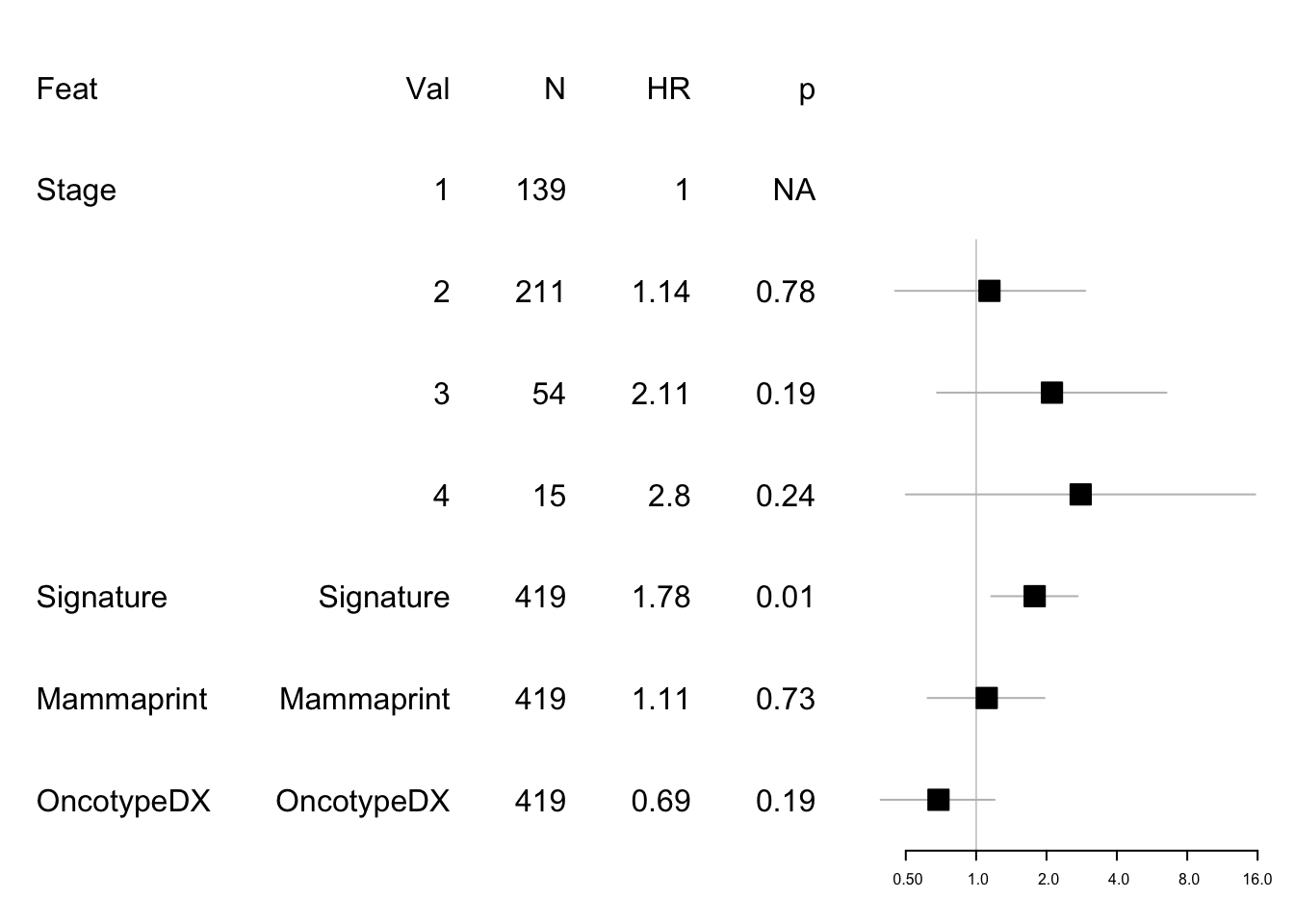
Next OS
data1=data.frame(Feat=c(  "Feat","Stage", "","","","Signature", "Mammaprint", "OncotypeDX"),
                Cat=c( "Val","1", "2", "3", "4","Signature", "Mammaprint","OncotypeDX"),
                N=c("N" ,table(newinfoTab$Stage), rep(nrow(newinfoTab), 3)),
                HR=c("HR",  1, round(summary(modelos)$coefficients[4:6, 2], 2), round(summary(modeldfs)$coefficients[1:3, 2], 2)),
                p=c("p" ,"NA", round(summary(modelos)$coefficients[4:6, 5], 2), round(summary(modeldfs)$coefficients[1:3, 5], 2)) )

mdata1=data.frame(rbind(NA,NA, round(summary(modelos)$conf.int[c(4:6, 1:3) ,c(1,3:4)], 2)))
#mdata=rbind(mdata, NA,  round(summary(modeldfs)$conf.int[4:6 ,c(1,3:4)], 2))

#pdf("figure-outputs/Figure5_CD74_forestplot.pdf", width=5, height=5)

forestplot(data1, mdata1, xlog=T,
           boxsize=0.2)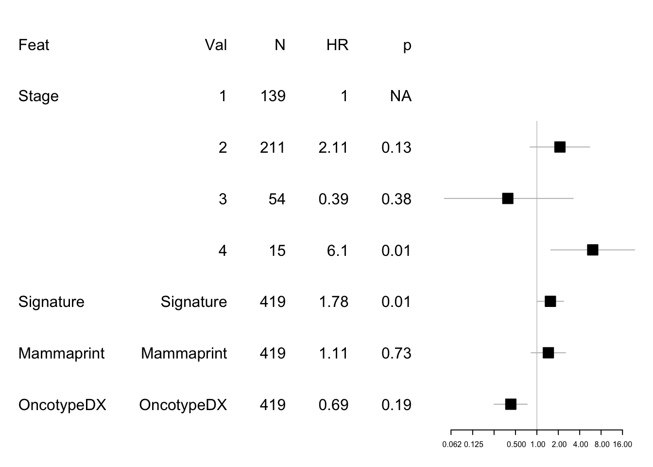
15.4.3 TCGA: LumA high vs low signatures
We can pull out the samples here which have high vs low signature (in the lumA group) and perform differential gene expression analysis on these cases:
newinfoTab$TCGAvalcut=cut(newinfoTab$TCGAgrow,  quantile(newinfoTab$TCGAgrow, c(0, 0.33, 0.67, 1) ), c("L", "M", "O"))
newinfoTab$TCGAvalcut[184]="L"

colDataTCGA=newinfoTab#[which(newinfoTab$TCGAvalcut!="M"), ]

TCGAdeseq=DESeqDataSetFromMatrix(round(TCGArsem2[ ,match(colDataTCGA$pat, colnames(TCGArsem2))]), colDataTCGA, design=~TCGAvalcut)

TCGAdeseq=DESeq(TCGAdeseq)

TCGAdeseqRes=results(TCGAdeseq, contrast=c("TCGAvalcut", "O", "L"))

#write.csv(TCGAdeseqRes, file="nature-tables/5J_TCGA.csv")

TCGAdeseqRes2=TCGAdeseqRes[which(TCGAdeseqRes$padj<0.05 & abs(TCGAdeseqRes$log2FoldChange)>1.5
                                 & TCGAdeseqRes$baseMean>100), ]

A1=as.data.frame(TCGAdeseqRes2)

DT::datatable(A1, rownames=T, class='cell-border stripe',
extensions="Buttons", options=list(dom="Bfrtip", buttons=c('csv', 'excel'), Xscroll=T))We can plot the differential genes here in a volcano plot:
#pdf("figure-outputs/Fig5J_TCGA_deg.pdf", height=8, width=8)
with(TCGAdeseqRes, plot(log2FoldChange, -log10(padj), pch=20, main="Volcano plot: Low exp (-) vs high (+)", cex=1.0, xlab=bquote(~Log[2]~fold~change), ylab=bquote(~-log[10]~Q~value)))
with(subset(TCGAdeseqRes, padj<0.05 & abs(log2FoldChange)>1.5 & baseMean>100), points(log2FoldChange, -log10(padj), pch=20, col="red", cex=0.5))
text(TCGAdeseqRes2$log2FoldChange+0.02, -log10(TCGAdeseqRes2$padj)+0.05, rownames(TCGAdeseqRes2))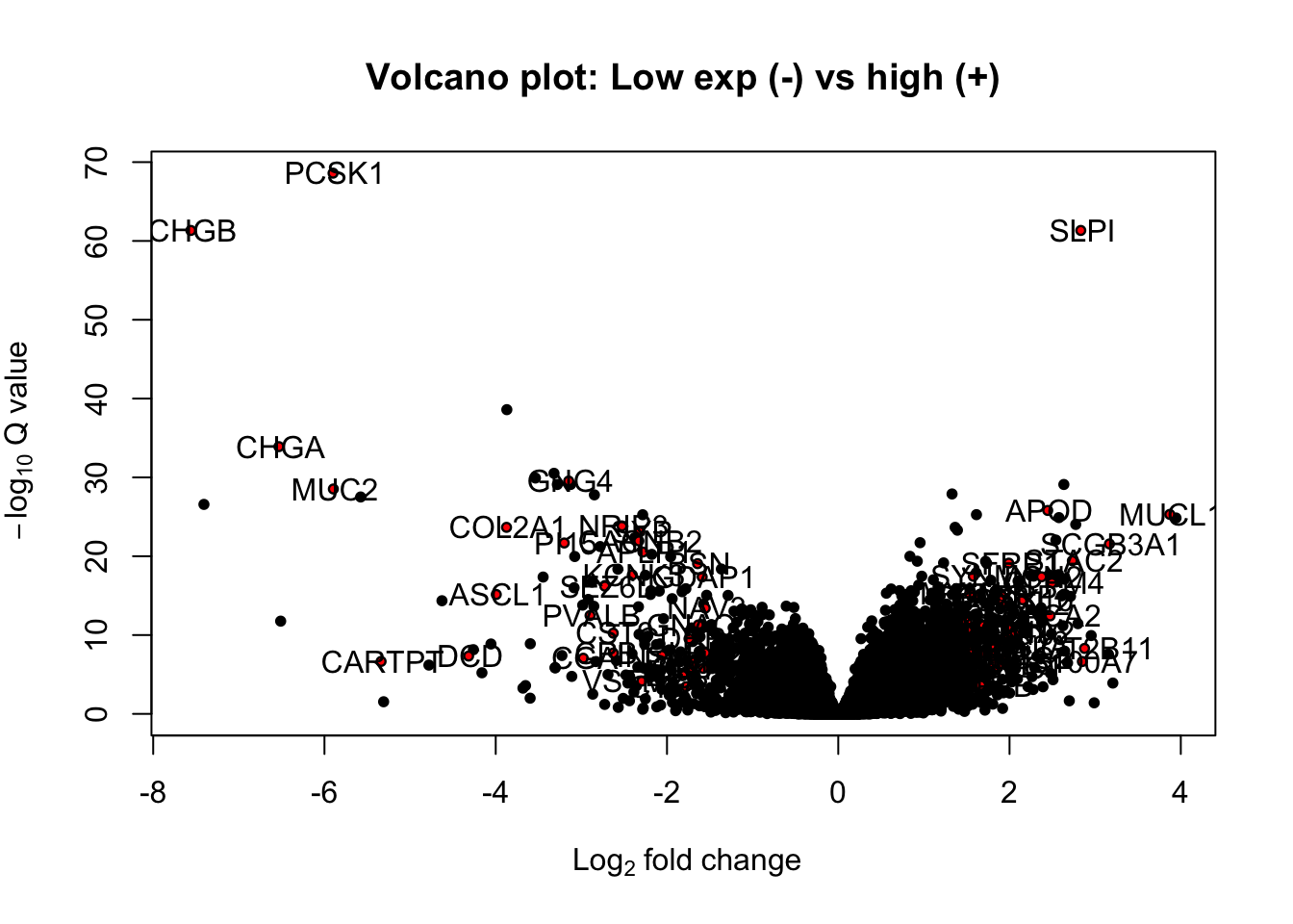
Figure 15.15: yet another volcano plot
#with(subset(TCGAdeseqRes, padj<0.05 & abs(log2FoldChange)>2), text(log2FoldChange+0.05, -log10(padj)+0.05, rownames(TCGAdeseqRes), pch=20, col="red", cex=0.75))
#dev.off()vstTCGA=vst(assay(TCGAdeseq))
ColSideCols=brewer.pal(3, "Blues")[factor(TCGAdeseq$TCGAvalcut)]
tx2=rownames(TCGAdeseqRes2)[which(rownames(TCGAdeseqRes2)%in%AllImmGenes)]
ax1=vstTCGA[ match(tx2, rownames(vstTCGA)), ]
heatmap.2(ax1, scale="row", trace="none", ColSideColors = ColSideCols, col=RdBu[11:1], main="LumA TCGA")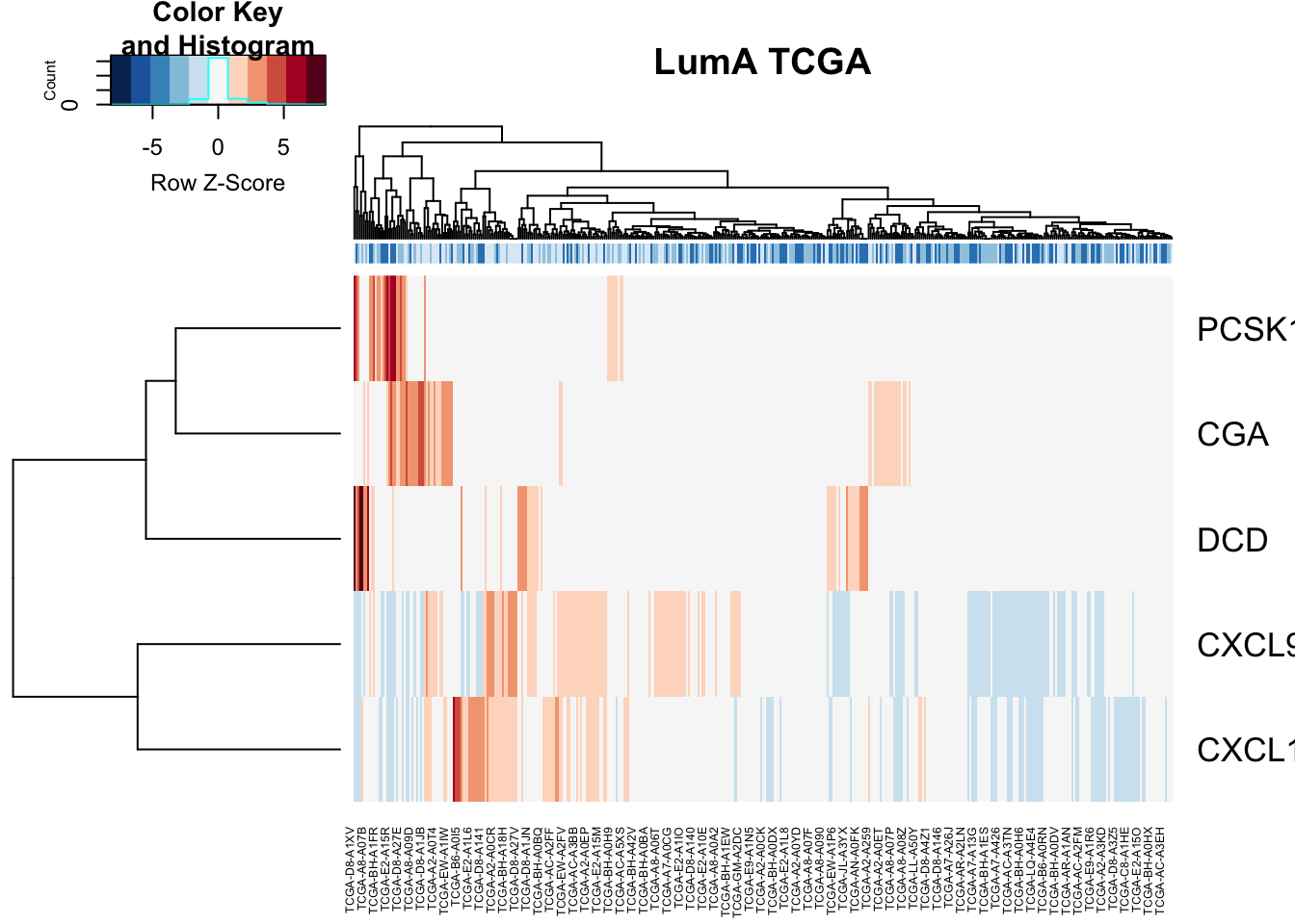
Figure 15.16: because someone will ask for it
#pdf("figure-outputs/Figure5J_XX_heatmap_LumA_TCGA.pdf", height=15, width=10)

heatmap.2(vstTCGA[ rownames(TCGAdeseqRes2),  ], scale="row", trace="none", ColSideColors = ColSideCols, col=RdBu[11:1], main="LumA TCGA")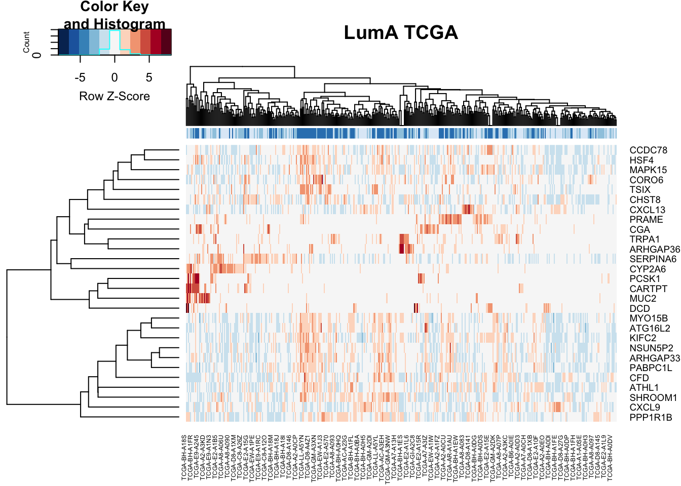
Figure 15.17: because someone will ask for it
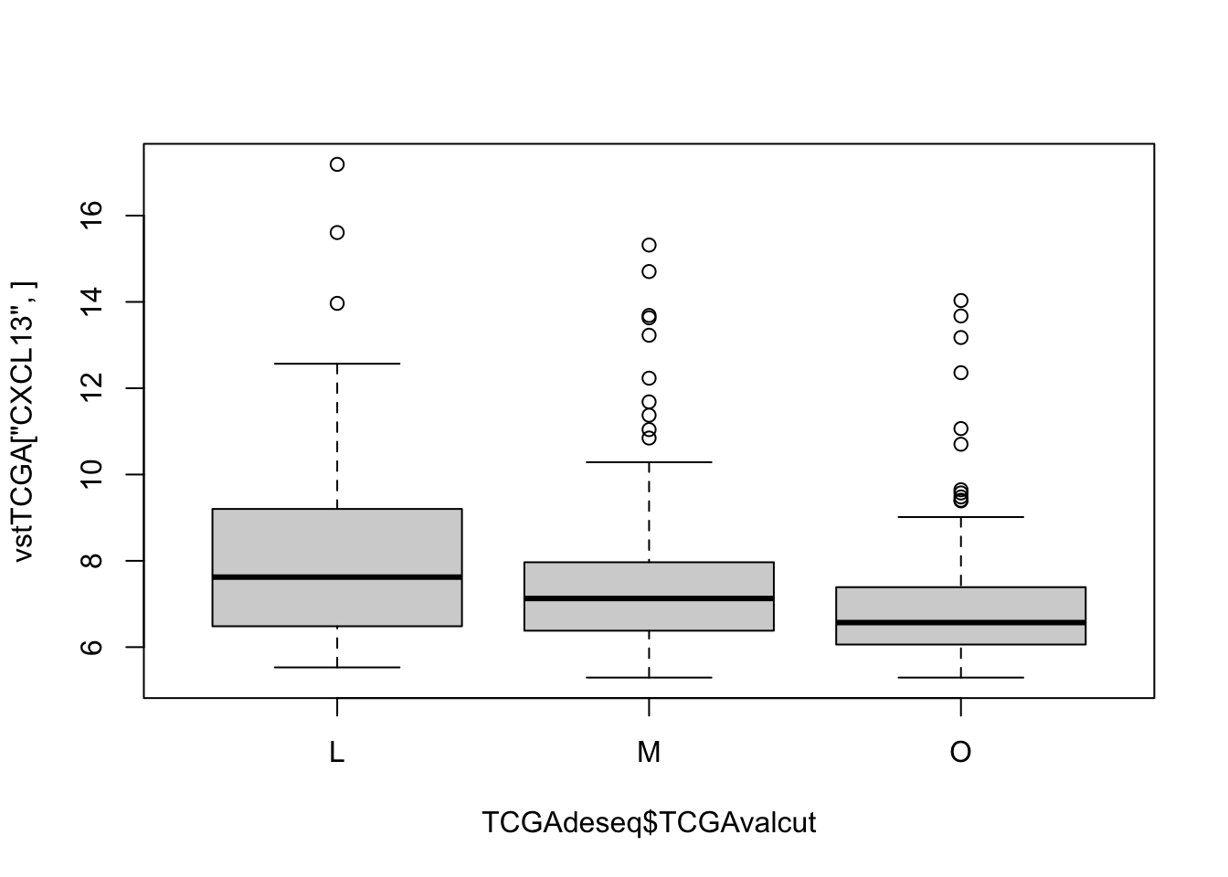
also check the directions by looking at CXCl13, which is an overexpressed gene:
Check if there is a difference in checkpoint proteins between the two:
ColSideCols=brewer.pal(3, "Blues")[factor(TCGAdeseq$TCGAvalcut[which(TCGAdeseq$TCGAvalcut!="M")])]
m1=match(unlist(ImmSuppAPC$Inh), rownames(vstTCGA))
m2=match(unlist(ImmSuppAPC$Act), rownames(vstTCGA))
m3=match(c("IFNG", "CTLA4", "GZMB"), rownames(vstTCGA))
ax1=vstTCGA[ na.omit(c(m1, m2, m3)),  which(TCGAdeseq$TCGAvalcut!="M")]
RowSideCols=c(rep("red", length(na.omit(m1))), rep("blue", length(na.omit(m2))), rep("forestgreen",3))

#pdf("figure-outputs/Figure5J_XX_heatmap_LumA_TCGA.pdf", height=15, width=10)

heatmap.2(ax1, scale="row", trace="none", ColSideColors = ColSideCols, col=RdBu[11:1], main="LumA TCGA" , RowSideColors = RowSideCols,hclustfun = hclust.ave, Rowv = NA)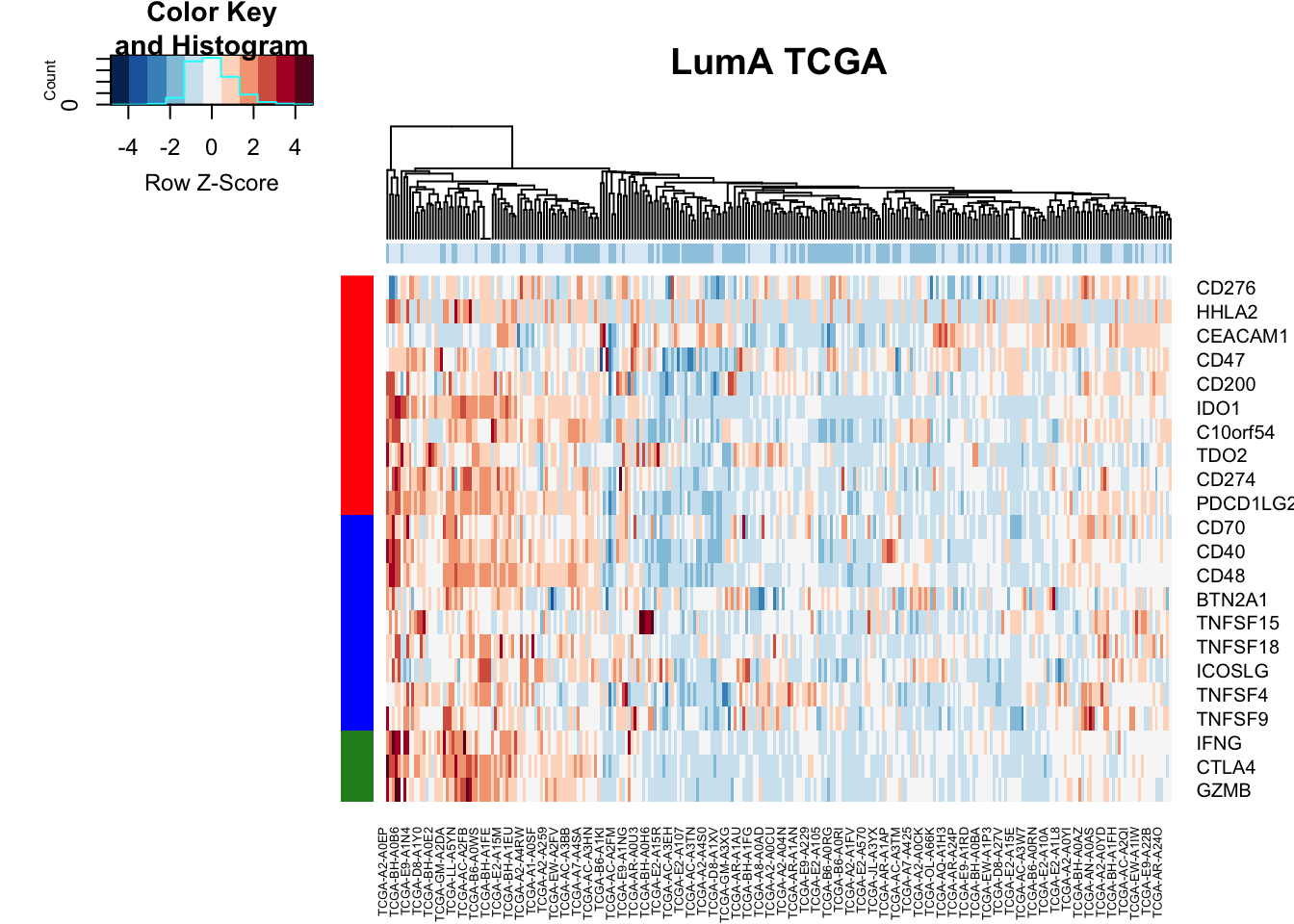
Run gsea here
hits=rownames(TCGAdeseqRes2)
fcTab=TCGAdeseqRes$log2FoldChange

names(fcTab)=rownames(TCGAdeseq)
  gscaTCGA=GSCA(listOfGeneSetCollections=ListGSC,geneList=fcTab, hits = hits)
   gscaTCGA<- preprocess( gscaTCGA, species="Hs", initialIDs="SYMBOL",
                    keepMultipleMappings=TRUE, duplicateRemoverMethod="max",
                    orderAbsValue=FALSE)
## -Preprocessing for input gene list and hit list ...
## --Removing genes without values in geneList ...
## --Removing duplicated genes ...
## --Converting annotations ...
## -- 2816 genes (out of 20060) could not be mapped to any identifier, and were removed from the data.
## -- 2 genes (out of 70) could not be mapped to any identifier, and were removed from the data.
## --Ordering Gene List decreasingly ...
## -Preprocessing complete!
   gscaTCGA <- analyze( gscaTCGA,
                 para=list(pValueCutoff=0.05, pAdjustMethod="BH",
                           nPermutations=100, minGeneSetSize=5,
                           exponent=1),
                           doGSOA = F)
## --21 gene sets don't have >= 5 overlapped genes with universe in gene set collection named c2List!
## --256 gene sets don't have >= 5 overlapped genes with universe in gene set collection named c5BP!
## --73 gene sets don't have >= 5 overlapped genes with universe in gene set collection named c5MF!
## --60 gene sets don't have >= 5 overlapped genes with universe in gene set collection named c5CC!
## --301 gene sets don't have >= 5 overlapped genes with universe in gene set collection named MetPathway!
## -Performing gene set enrichment analysis using HTSanalyzeR2...
## --Calculating the permutations ...
## -Gene set enrichment analysis using HTSanalyzeR2 complete
## ==============================================

save( gscaTCGA, file="figure-outputs/TCGA_hairball.RData")

TermsA=sapply(strsplit(rownames(gscaTCGA@result$GSEA.results$ProcessNetworks), "_"), function(x) x[2])
TermsA[which(is.na(TermsA))]=substr(rownames(gscaTCGA@result$GSEA.results$ProcessNetworks)[which(is.na(TermsA))], 2, 50)

## check whether this runs:
gscaTCGA@result$GSEA.results$ProcessNetworks$Gene.Set.Term=TermsA
viewEnrichMap(gscaTCGA, gscs=c("ProcessNetworks"),
              allSig = TRUE, gsNameType="term" )
Figure 15.18: pointless TCGA hairball