Chapter 14 Epcam+ Inflammatory vs non-inflammatory samples
14.1 Identification of inflammatory samples
Here, look at individual enrichment scores (ssGSEA). We notice in the Epithelial samples there are 5 samples which appear to be hyperinflammatory: They have higher enrichment for TNFA, interferon signalling for example.
d1=DNismr3$Hallmark[, c("stable_vs_growing NES", "stable_vs_growing padj")]
e1=Epismr3$Hallmark[, c("stable_vs_growing NES", "stable_vs_growing padj")]
c1=CDismr3$Hallmark[, c("stable_vs_growing NES", "stable_vs_growing padj")]
#
ds=which(d1[ ,2]<0.05)
es=which(e1[ ,2]<0.05)
cs=which(c1[ ,2]<0.05)

AUnique=c(rownames(d1)[ds], rownames(e1)[es], rownames(c1)[cs])
xalist=unique(AUnique)

sList=PathInH[match((rownames(e1)[es]), names(PathInH))]

tpmTemp=allTPMFinal[ , match(vstEp$SampleID, colnames(allTPMFinal))]
colnames(tpmTemp)=infoTableFinal$TumorIDnew[match(colnames(tpmTemp), rownames(infoTableFinal))]
rownames(tpmTemp)=rNames2

gsva1=gsva(tpmTemp, sList, method="ssgsea", ssgsea.norm=T)

nx2=sapply(1:nrow(gsva1), function(x) sd(gsva1[x, ]))
a1=which(nx2>0.03)

sList=PathInH[match((rownames(d1)[ds]), names(PathInH))]

tpmTemp=allTPMFinal[ , match(vstDN$SampleID, colnames(allTPMFinal))]
colnames(tpmTemp)=infoTableFinal$TumorIDnew[match(colnames(tpmTemp), rownames(infoTableFinal))]
rownames(tpmTemp)=rNames2

gsva2=gsva(tpmTemp, sList, method="ssgsea", ssgsea.norm=T)

nx2=sapply(1:nrow(gsva2), function(x) sd(gsva2[x, ]))
a2=which(nx2>0.03)

sList=PathInH[match((rownames(c1)[cs]), names(PathInH))]

tpmTemp=allTPMFinal[ , match(vstCD$SampleID, colnames(allTPMFinal))]
rownames(tpmTemp)=rNames2

gsva3=gsva(tpmTemp, sList, method="ssgsea", ssgsea.norm=T)

nx2=sapply(1:nrow(gsva3), function(x) sd(gsva3[x, ]))
a3=which(nx2>0.03)

#pdf("~/Desktop/5B-ssgsea-scores-hallmark-pathways.pdf", height=5, width=5)

HRstat2=Cdata$HR_status[match(vstEp$TumorID, Cdata$TumorID)]
HRstat2[which(HRstat2=="Basal")]=NA
Check which pathways are enriched in which specific samples:
par(oma=c(1, 1, 1, 5))
# heatmap.2(gsva1[a1, ], col=RdBu[11:1], scale="none", trace="none", ColSideColors = ColSizeb[vstEp$Growth],
#           main="Ep")
heatmap.2(gsva1[a1, ], col=RdBu[11:1], scale="none", trace="none", ColSideColors = ColMerge[ vstEp$Treatment,1],
          main="Ep")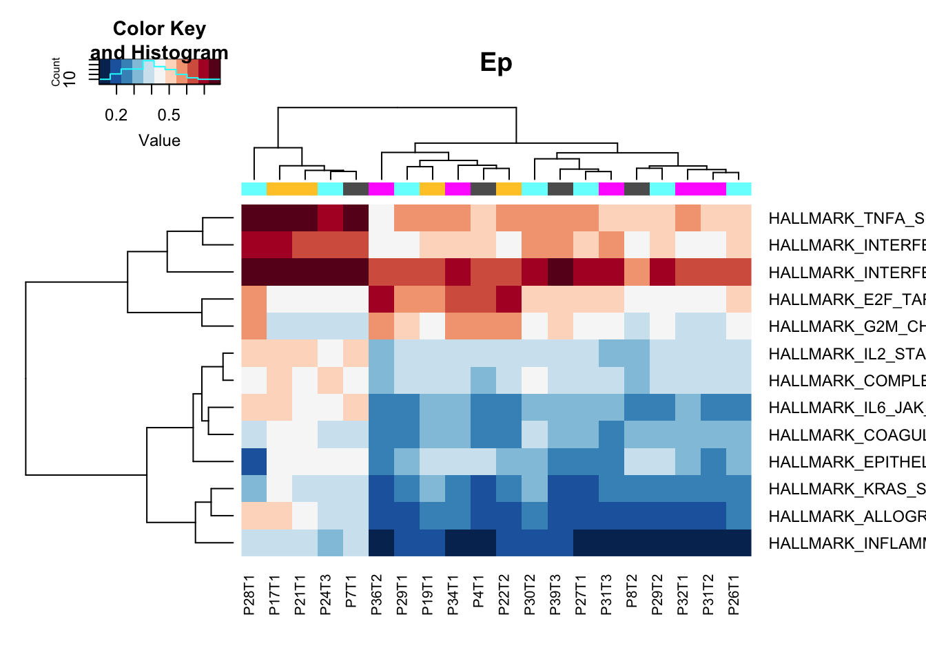
Figure 14.1: ssGSEA specific pathways
Below are the pathways specific to cd45 and dn
heatmap.2(gsva2[a2, ], col=RdBu[11:1], scale="none", trace="none", ColSideColors = ColSizeb[vstDN$Growth],
          main="DN")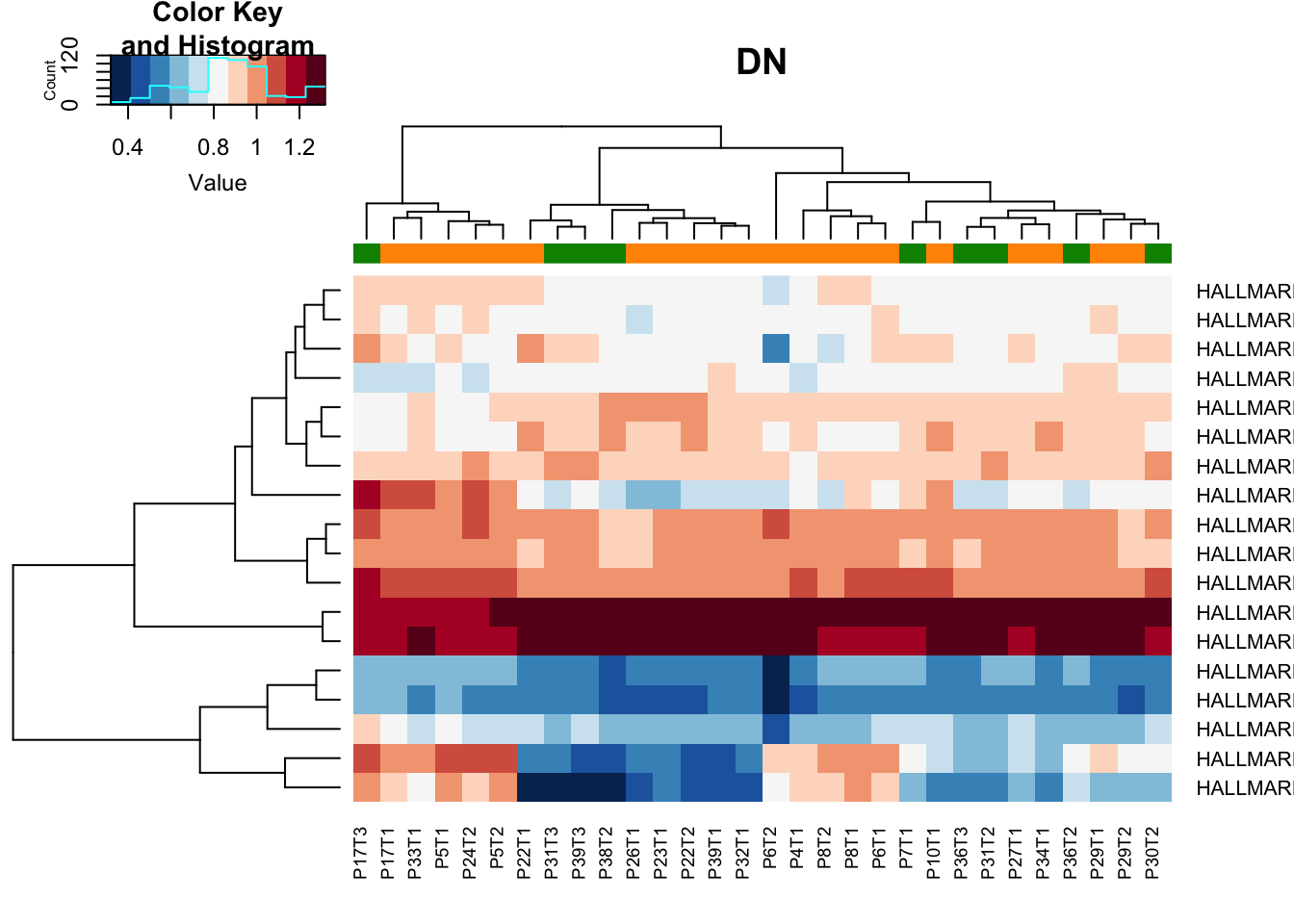
heatmap.2(gsva3[a3, ], col=RdBu[11:1], scale="none", trace="none", ColSideColors = ColSizeb[vstCD$Growth],
          main="CD")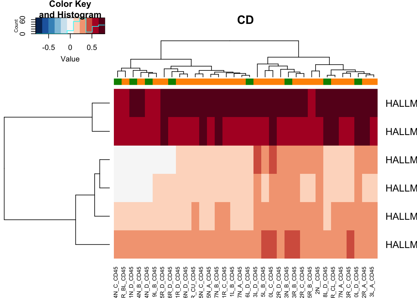
14.2 DEG: inflammatory vs non-inflammatory
What genes are different between inflammatory and non-inflammatory?
Inflamm=c("11N_D_Ep", "6R_B_Ep", "8L_D_Ep", "10L_D_Ep", "3N_B_Ep")

Epdds$Inflammation="no"
Epdds$Inflammation[which(colnames(Epdds)%in%Inflamm)]="yes"
Epdds$Inflammation=factor(Epdds$Inflammation)


vstEpInf=Epdds
design(vstEpInf)=~Inflammation
vstEpInf=DESeq(vstEpInf)

vstEpInfRes=results(vstEpInf)

sigGenes=rownames(vstEpInfRes)[which(vstEpInfRes$padj<0.05 & abs(vstEpInfRes$log2FoldChange)>2.5 &
                 vstEpInfRes$baseMean>200)]

#colnames(vstEp)=infoTableFinal$TumorIDnew[match(colnames(vstEp), rownames(infoTableFinal))]

heatmap.2(assay(vstEp)[sigGenes, ], col=RdBu[11:1], trace="none", scale = "row", ColSideColors = ColSizeb[vstEpInf$Growth], hclustfun = hclust.ave)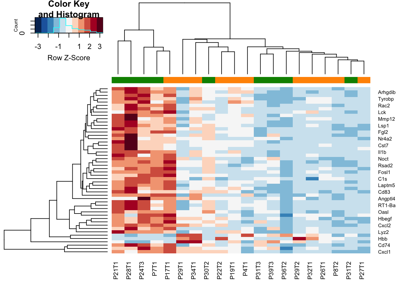
Figure 14.2: Differential gene exp inflammatory vs non-inflammatory
#write.csv(assay(vstEp)[sigGenes, ], file="nature-tables/Ext5c_heatmap.csc")

DT::datatable(as.data.frame(vstEpInfRes[sigGenes, ]), rownames=F, class='cell-border stripe',
          extensions="Buttons", options=list(dom="Bfrtip", buttons=c('csv', 'excel')))
Figure 14.2: Differential gene exp inflammatory vs non-inflammatory
There are 27 genes which differentiates these two, which includes Csf3, Ccl22, Ccl3, Pltp, Lck, Rac2, Mmp12, Rsad2, Bcl2a1, Cxcl1, Lyz2, C1s, Ccl2, Nr4a2, Plaur, Ets1, Plau, Angptl4, Il1b, Cxcl2, Hbegf, Cd74, Ccl17, Thbs1, RT1-Da, Oasl, Tyrobp.
We can also assess whether there is an association between immune infiltration. We can compare whether the non-inflammatory have differences in T-cell infiltration, mixing indices based on imaging data. Below ‘no’ samples are non-inflammatory and ‘yes’ samples are hyper-inflammatory.
## boxplots for
nTab=data.frame(inf=vstEpInf$Inflammation, MH=vstEpInf$MHEpCAM, cd8=vstEpInf$CD8Frac,
           knn=vstEpInf$knnEpCAM)
nTabmelt=melt(nTab, measure.vars = c("cd8", "knn", "MH"))

ggplot(data=nTabmelt, aes(x=inf, y=value))+geom_boxplot()+geom_point()+theme_bw()+facet_wrap(~variable, scale="free")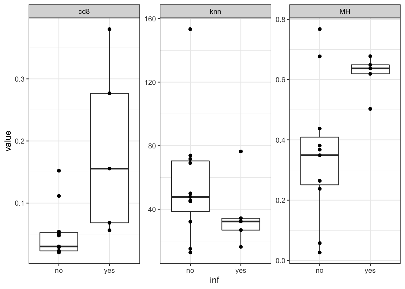
Figure 14.3: association signature with WSI
#write.csv(nTabmelt, file="nature-tables/Ext5d.csv")

Cdata$Inflammation=NA
Cdata$Inflammation=vstEpInf$Inflammation2[match(Cdata$NewID, colnames(vstEp))]

DT::datatable(nTab, rownames=F, class='cell-border stripe',
          extensions="Buttons", options=list(dom="Bfrtip", buttons=c('csv', 'excel')))
Figure 14.3: association signature with WSI
Statistics are below:
print('assoc with cd8')
## [1] "assoc with cd8"
t.test(nTab$cd8~nTab$inf)
##
##  Welch Two Sample t-test
##
## data:  nTab$cd8 by nTab$inf
## t = -2.141, df = 4.3454, p-value = 0.09351
## alternative hypothesis: true difference in means is not equal to 0
## 95 percent confidence interval:
##  -0.30731448  0.03501129
## sample estimates:
##  mean in group no mean in group yes
##        0.05119239        0.18734398
#table(nTab$cd8, nTab$inf)
print('assoc with MH index')
## [1] "assoc with MH index"
t.test(nTab$MH~nTab$inf)
##
##  Welch Two Sample t-test
##
## data:  nTab$MH by nTab$inf
## t = -3.6191, df = 13.053, p-value = 0.003096
## alternative hypothesis: true difference in means is not equal to 0
## 95 percent confidence interval:
##  -0.4295016 -0.1084920
## sample estimates:
##  mean in group no mean in group yes
##         0.3482039         0.6172007
#table(nTab$MH,nTab$inf)
print('assoc with knn')
## [1] "assoc with knn"
t.test(nTab$knn~nTab$inf)
##
##  Welch Two Sample t-test
##
## data:  nTab$knn by nTab$inf
## t = 1.2134, df = 12.512, p-value = 0.2474
## alternative hypothesis: true difference in means is not equal to 0
## 95 percent confidence interval:
##  -14.76130  52.25308
## sample estimates:
##  mean in group no mean in group yes
##          56.00313          37.25724
#table(nTab$knn~nTab$inf)
14.3 Finding 3 signatures for 3 branches
Below we can perform a 1 vs all analysis i.e. compare
- growing vs the rest
- inflammatory vs the rest
- stable vs the rest
#vstEpInf$Inflammation2=vstEpInf$Inflammation
vstEpInf$Inflammation2=factor(ifelse(vstEpInf$Inflammation=="yes", "inf", ifelse(vstEpInf$Growth=="growing", "grow", "stab")))


design(vstEpInf)=~Inflammation2
vstEpInf=DESeq(vstEpInf)

vstEpInfRes1=results(vstEpInf, contrast = c("Inflammation2", "stab", "inf"))
res1genes=rownames(vstEpInfRes1)[which(vstEpInfRes1$padj<0.05 & abs(vstEpInfRes1$log2FoldChange)>1.5 &
                                         vstEpInfRes1$baseMean>100)]

vstEpInfRes2=results(vstEpInf, contrast = c("Inflammation2", "stab", "grow"))
res2genes=rownames(vstEpInfRes2)[which(vstEpInfRes2$padj<0.05 & abs(vstEpInfRes2$log2FoldChange)>1.5 &
                                         vstEpInfRes2$baseMean>100)]

vstEpInfRes3=results(vstEpInf, contrast = c("Inflammation2", "grow", "inf"))
res3genes=rownames(vstEpInfRes3)[which(vstEpInfRes3$padj<0.05 & abs(vstEpInfRes3$log2FoldChange)>1.5 &
                                         vstEpInfRes3$baseMean>100)]

aUnique=c(res1genes, res2genes, res3genes)

AX1=setdiff(res2genes, res1genes)
ax2=setdiff(res3genes, res1genes)

heatmap.2(assay(vstEp)[AX1, ], col=RdBu[11:1], trace="none", scale = "row", ColSideColors = ColSizec[vstEpInf$Inflammation2], hclustfun = hclust.ave)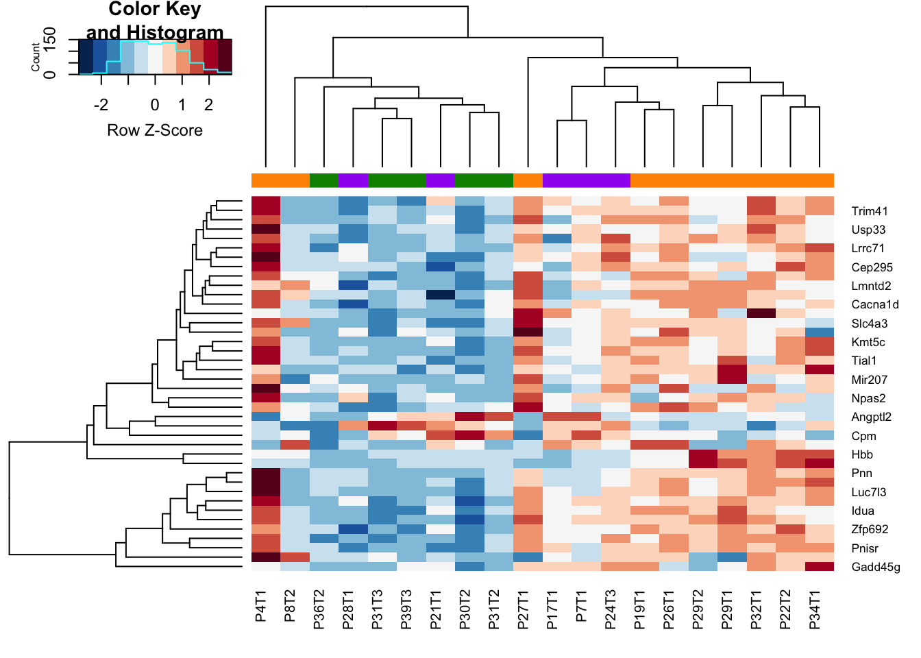
write.csv(assay(vstEp)[AX1, ], file="nature-tables/Ext5c.csv")

nTab=data.frame(inf=vstEpInf$Inflammation2, MH=vstEpInf$MHEpCAM, cd8=vstEpInf$CD8Frac,
           knn=vstEpInf$knnEpCAM)
nTabmelt=melt(nTab, measure.vars = c("cd8", "knn", "MH"))

ggplot(data=nTabmelt, aes(x=inf, y=value))+geom_boxplot()+geom_point()+theme_bw()+facet_wrap(~variable, scale="free")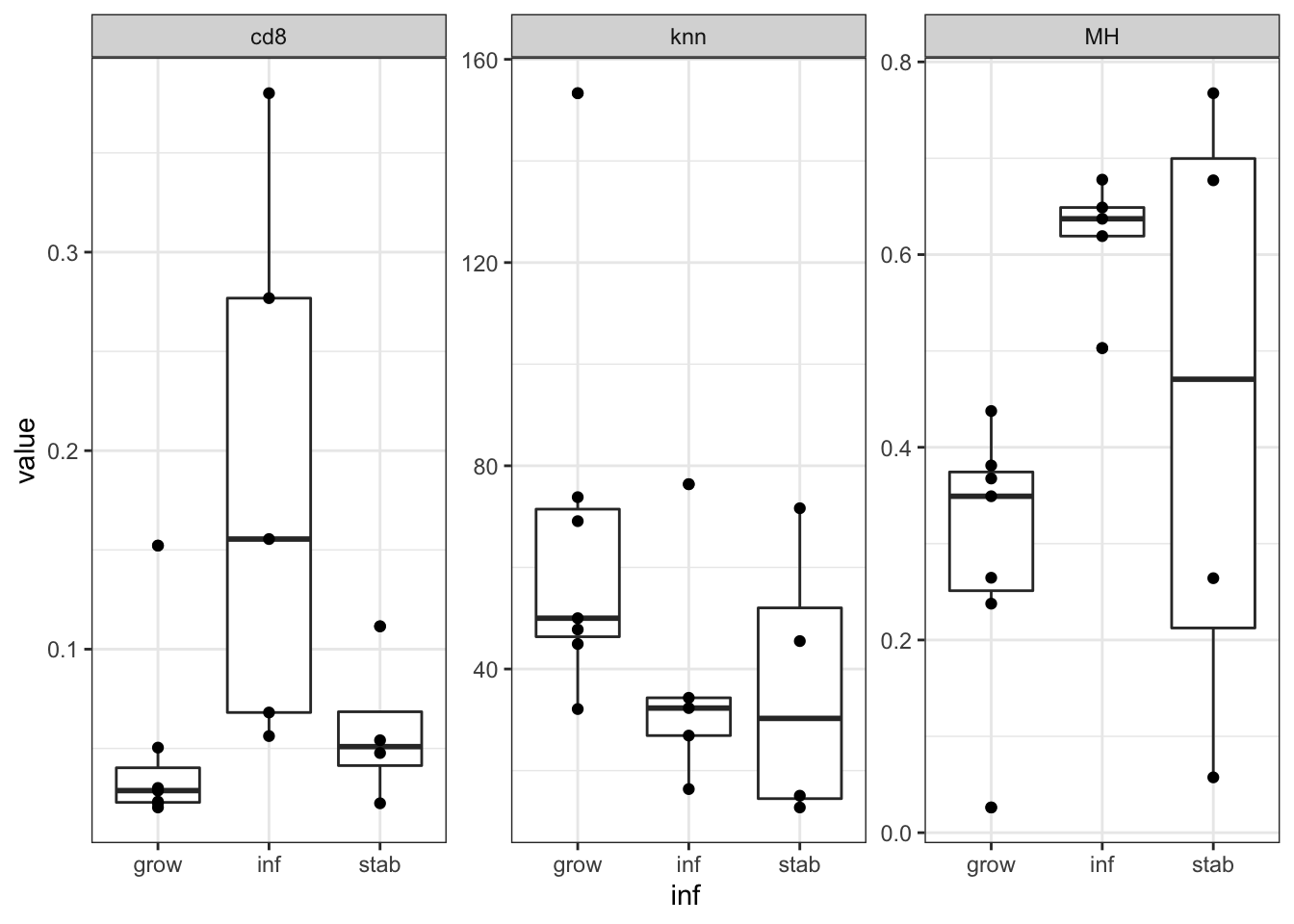
We see that the growing vs stable samples are very similary overall, however, DEGs between growing and stable are also expressed in the inflammatory branch.
We can use these gene signatures to identify each branch: Below, we see the separation between the 3 groups using these genes. (note that the stable branch has no identifiable upregulated genes and is defined by the negative score of the downregulated genes:). We use ssGSEA to get a score for each sample
vstEpInf$Inflammation3=vstEpInf$Inflammation2
vstEpInf$Inflammation3[which(vstEpInf$Inflammation3=="stab")]="inf"
vstEpInf$Inflammation3=factor(vstEpInf$Inflammation3)
design(vstEpInf)=~(Inflammation3)
vstEpInfb=DESeq(vstEpInf)
vstEpInfRes1b=results(vstEpInfb)
res1genesGrow=rownames(vstEpInfRes1b)[which(vstEpInfRes1b$padj<0.05 & (vstEpInfRes1b$log2FoldChange)<(-1.5) &
vstEpInfRes1b$baseMean>100)]
vstEpInf$Inflammation3=vstEpInf$Inflammation2
vstEpInf$Inflammation3[which(vstEpInf$Inflammation2=="grow")]="inf"
vstEpInf$Inflammation3=factor(vstEpInf$Inflammation3)
design(vstEpInf)=~(Inflammation3)
vstEpInfb=DESeq(vstEpInf)
vstEpInfRes1b=results(vstEpInfb)
res1genesStab=rownames(vstEpInfRes1b)[which(vstEpInfRes1b$padj<0.05 & (vstEpInfRes1b$log2FoldChange)<(-1.5) &
vstEpInfRes1b$baseMean>100)]
vstEpInf$Inflammation3=vstEpInf$Inflammation2
vstEpInf$Inflammation3[which(vstEpInf$Inflammation2=="stab")]="grow"
vstEpInf$Inflammation3=factor(vstEpInf$Inflammation3)
design(vstEpInf)=~(Inflammation3)
vstEpInfb=DESeq(vstEpInf)
vstEpInfRes1b=results(vstEpInfb)
res1genesInf=rownames(vstEpInfRes1b)[which(vstEpInfRes1b$padj<0.05 & (vstEpInfRes1b$log2FoldChange)>(1.5) &
vstEpInfRes1b$baseMean>100)]
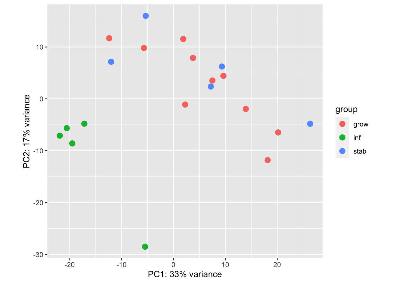
## perform ssGSEA on these samples and see where they fit:
RatssGSEA=gsva(assay(vsdLimmaEp),
list(grow=res1genesGrow, inh=res1genesInf, nonstab=res1genesStab), method="ssgsea", ssgsea.norm=T)
par(mfrow=c(1,2))
plot(RatssGSEA[1, ], RatssGSEA[2, ], col=factor(vstEpInf$Inflammation2), xlab="grow score", ylab="inh score")
plot(RatssGSEA[1, ], -RatssGSEA[3, ], col=factor(vstEpInf$Inflammation2), xlab="grow score", ylab="-stab score")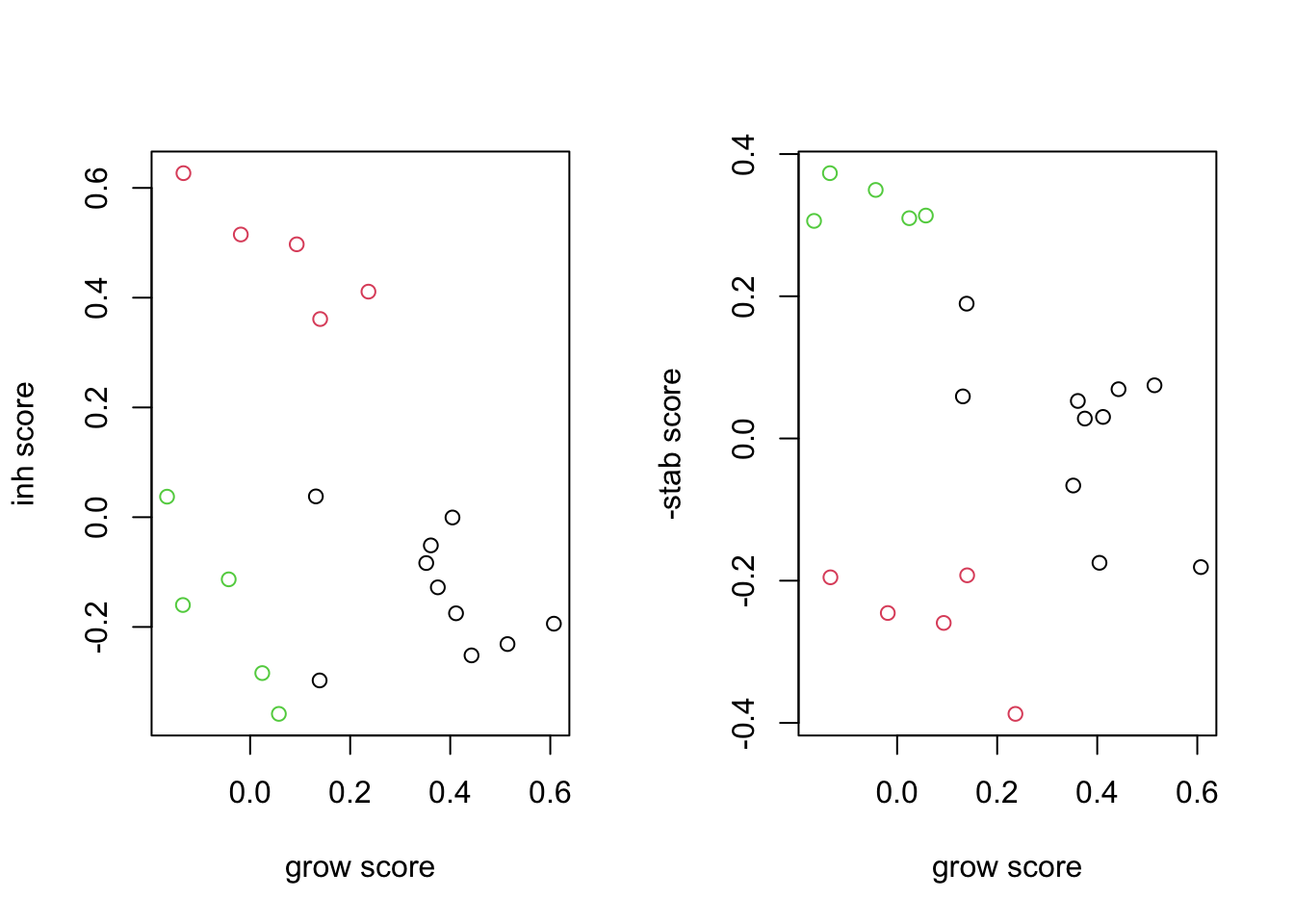
We can also overlay these signatures from ssGSEA to see how well it can predict each group:
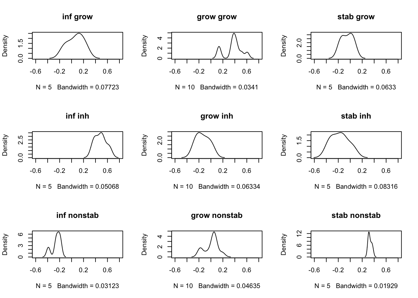
# plot histograms for the 3 samples:
par(mfrow=c(3,3))

for (i in 1:3){
  for (j in c("inf", "grow", "stab")){
    plot(density(RatssGSEA[i, which(vstEpInf$Inflammation2==j)]), main=paste(j, rownames(RatssGSEA)[i]),
         xlim=c(-0.6, 0.8))
  }
}
GSEA for the above 3 groups?
load("../anntotations/ListofGeneSets2.RData")

l1=SymHum2Rat$HGNC.symbol[match(rownames(vstEpInfRes1), SymHum2Rat$RGD.symbol)]
l2=Rat2Hum$HGNC.symbol[match(rownames(vstEpInfRes1), Rat2Hum$RGD.symbol)]
l3=Mouse2Hum$HGNC.symbol[match(rownames(vstEpInfRes1), Mouse2Hum$MGI.symbol)]
EpGenesConv=ifelse(is.na(l1)==F, l1, ifelse(is.na(l2)==F, l2, ifelse(is.na(l3)==F, l3, rownames(vstEpInfRes1))))

##
## run 1
hits=EpGenesConv[match(res1genes, rownames(vstEpInfRes1))]
fcTab=vstEpInfRes1$log2FoldChange
names(fcTab)=EpGenesConv
  gscaepInf1=GSCA(listOfGeneSetCollections=ListGSC,geneList=fcTab, hits = hits)
  gscaepInf1 <- preprocess(gscaepInf1, species="Hs", initialIDs="SYMBOL",
                    keepMultipleMappings=TRUE, duplicateRemoverMethod="max",
                    orderAbsValue=FALSE)
  gscaepInf1 <- analyze(gscaepInf1,
                 para=list(pValueCutoff=0.05, pAdjustMethod="BH",
                           nPermutations=100, minGeneSetSize=5,
                           exponent=1),
                           doGSOA = F)
## run2
hits=EpGenesConv[match(res2genes, rownames(vstEpInfRes2))]
fcTab=vstEpInfRes2$log2FoldChange
names(fcTab)=EpGenesConv
gscaepInf2=GSCA(listOfGeneSetCollections=ListGSC,geneList=fcTab, hits = hits)
gscaepInf2 <- preprocess(gscaepInf2, species="Hs", initialIDs="SYMBOL",
                    keepMultipleMappings=TRUE, duplicateRemoverMethod="max",
                    orderAbsValue=FALSE)
gscaepInf2 <- analyze(gscaepInf2,
                 para=list(pValueCutoff=0.05, pAdjustMethod="BH",
                           nPermutations=100, minGeneSetSize=5,
                           exponent=1),
                           doGSOA = F)
## run3
hits=EpGenesConv[match(res3genes, rownames(vstEpInfRes3))]
fcTab=vstEpInfRes3$log2FoldChange
names(fcTab)=EpGenesConv
gscaepInf3=GSCA(listOfGeneSetCollections=ListGSC,geneList=fcTab, hits = hits)
gscaepInf3 <- preprocess(gscaepInf3, species="Hs", initialIDs="SYMBOL",
                    keepMultipleMappings=TRUE, duplicateRemoverMethod="max",
                    orderAbsValue=FALSE)
gscaepInf3 <- analyze(gscaepInf3,
                 para=list(pValueCutoff=0.05, pAdjustMethod="BH",
                           nPermutations=100, minGeneSetSize=5,
                           exponent=1),
                           doGSOA = F)


GSEA1=gscaepInf1@result$GSEA.results$ProcessNetworks
GSEA2=gscaepInf2@result$GSEA.results$ProcessNetworks
GSEA3=gscaepInf3@result$GSEA.results$ProcessNetworks

tempOut=cbind(GSEA1, GSEA2, GSEA3, file="nature-tables/Supp3_output_GSEA_tables_growing_stable.csv")

lx1=unique(c(rownames(GSEA1)[which(GSEA1[ ,3]<0.05)],
      rownames(GSEA2)[which(GSEA2[ ,3]<0.05)],
      rownames(GSEA3)[which(GSEA3[ ,3]<0.05)]))


Fx=cbind(GSEA1[lx1, 1], GSEA3[lx1, 1], GSEA2[lx1, 1])
Fx2=cbind(GSEA1[lx1, 3], GSEA3[lx1, 3], GSEA2[lx1, 3])
Fx[which(Fx2>0.05, arr.ind=T)]=0

rownames(Fx)=lx1
colnames(Fx)=c("s/i", "g/i", "s/g")


ltest=which(rowSums(sign(abs(Fx)))>1)
ltest2=which(abs(Fx[,3])>0)

par(oma=c(1,1,1,5))
heatmap.2(Fx[unique(c(ltest,ltest2)), ], col=RdBu[11:1], trace="none", scale = "none", hclustfun = hclust.ave)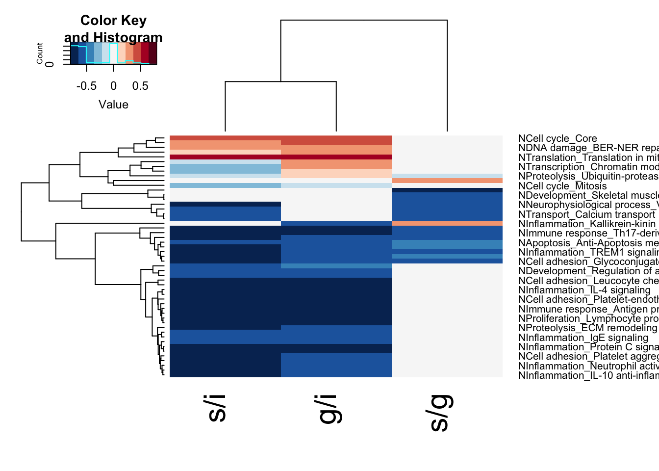
14.4 Analyse the non-inflammatory samples
We remove all the inflammtory samples and compare differences between stable and growing here. Below is the volcano plot for the
#Remove inflammatory samples
#Also remove samples which are basal-like

Inflamm=c("11N_D_Ep", "6R_B_Ep", "8L_D_Ep", "10L_D_Ep", "3N_B_Ep") #,"2N__Ep", "15N_C_Ep", "7N_A_Ep", "8R_CU_Ep", "12L_D_Ep", "14N_D_Ep")

EpddsInflam=EpddsGrowth
EpddsInflam=EpddsInflam[, -match(Inflamm, colnames(EpddsInflam))]
#design(EpddsInflam)=~Growth
EpddsInflam=DESeq(EpddsInflam)

ResA=results(EpddsInflam, contrast = c("Growth", "stable", "growing"))
ResAb=ResA[which(ResA$padj<0.05 & abs(ResA$log2FoldChange)>1.5 & ResA$baseMean>100), ]


#pdf("~/Desktop/5C-heatmap-inflamm-vs-non-inflamm-lowexpressing-included.pdf", width=8, height=12)

plot(ResA$log2FoldChange, -log10(ResA$padj), pch=20, col="black",
     main="growing (-ve) vs stable (+ve)")

text(ResAb$log2FoldChange, -log10(ResAb$padj), rownames(ResAb), col="red")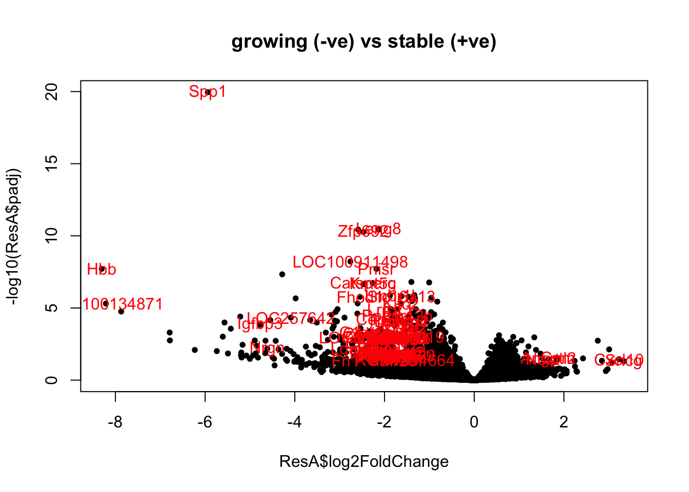
Figure 14.4: ep non-inflammatory comparison
Followed by the heatmap for this analysis
vst2=vst(EpddsInflam)

heatmap.2(assay(vst2)[match(rownames(ResAb), rownames(vst2)), ], col=RdBu[11:1],
          ColSideColors = ColSizeb[vst2$Growth], trace="none", scale="row")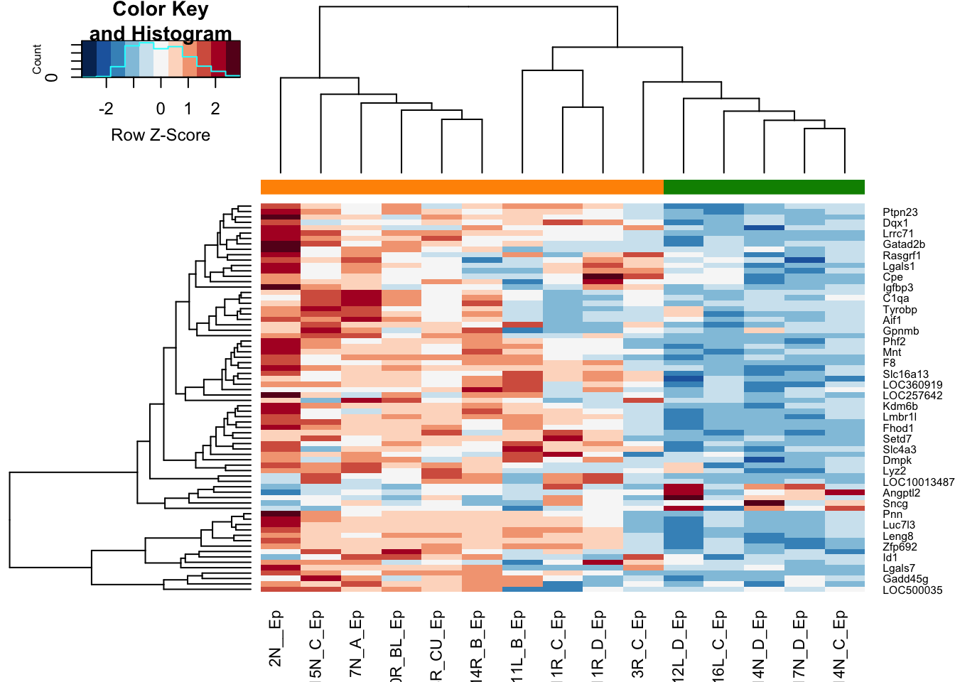
Figure 14.5: ep non-inflammatory comparison heatmap
14.4.1 GSEA
Quickly run GSEA for these samples:
EpGenes=rownames(ResA)

l1=SymHum2Rat$HGNC.symbol[match(EpGenes, SymHum2Rat$RGD.symbol)]
l2=Rat2Hum$HGNC.symbol[match(EpGenes, Rat2Hum$RGD.symbol)]
l3=Mouse2Hum$HGNC.symbol[match(EpGenes, Mouse2Hum$MGI.symbol)]
EpGenesConv=ifelse(is.na(l1)==F, l1, ifelse(is.na(l2)==F, l2, ifelse(is.na(l3)==F, l3, EpGenes)))


hits=EpGenesConv[match(rownames(ResAb), EpGenes)]
fcTab=ResA$log2FoldChange
names(fcTab)=EpGenesConv


  gscaepInf=GSCA(listOfGeneSetCollections=ListGSC,geneList=fcTab, hits = hits)
  gscaepInf <- preprocess(gscaepInf, species="Hs", initialIDs="SYMBOL",
                    keepMultipleMappings=TRUE, duplicateRemoverMethod="max",
                    orderAbsValue=FALSE)
## -Preprocessing for input gene list and hit list ...
## --Removing genes without values in geneList ...
## --Removing duplicated genes ...
## --Converting annotations ...
## -- 527 genes (out of 12341) could not be mapped to any identifier, and were removed from the data.
## -- 7 genes (out of 72) could not be mapped to any identifier, and were removed from the data.
## --Ordering Gene List decreasingly ...
## -Preprocessing complete!
  gscaepInf <- analyze(gscaepInf,
                 para=list(pValueCutoff=0.05, pAdjustMethod="BH",
                           nPermutations=100, minGeneSetSize=5,
                           exponent=1),
                           doGSOA = F)
## --146 gene sets don't have >= 5 overlapped genes with universe in gene set collection named c2List!
## --848 gene sets don't have >= 5 overlapped genes with universe in gene set collection named c5BP!
## --269 gene sets don't have >= 5 overlapped genes with universe in gene set collection named c5MF!
## --110 gene sets don't have >= 5 overlapped genes with universe in gene set collection named c5CC!
## --377 gene sets don't have >= 5 overlapped genes with universe in gene set collection named MetPathway!
## -Performing gene set enrichment analysis using HTSanalyzeR2...
## --Calculating the permutations ...
## -Gene set enrichment analysis using HTSanalyzeR2 complete
## ==============================================

A1=HTSanalyzeR2::summarize(gscaepInf)
##
## -No of genes in Gene set collections:
##                 input above min size
## c2List           2199           2053
## c5BP             7530           6682
## c5MF             1663           1394
## c5CC              999            889
## ProcessNetworks   158            158
## MetPathway       1480           1103
## Hallmark           50             50
##
##
## -No of genes in Gene List:
##           input valid duplicate removed converted to entrez
## Gene List 12449 12449             12341               11814
##
##
## -No of hits:
##      input preprocessed
## Hits    72           65
##
##
## -Parameters for analysis:
##               minGeneSetSize pValueCutoff pAdjustMethod
## HyperGeo Test 5              0.05         BH
##
##      minGeneSetSize pValueCutoff pAdjustMethod nPermutations exponent
## GSEA 5              0.05         BH            100           1
##
##
## -Significant gene sets (adjusted p-value< 0.05 ):
##          c2List c5BP c5MF c5CC ProcessNetworks MetPathway Hallmark
## HyperGeo     NA   NA   NA   NA              NA         NA       NA
## GSEA        188  641  116  130              17         16       19
## Both         NA   NA   NA   NA              NA         NA       NA

PNresultsef=gscaepInf@result$GSEA.results$ProcessNetworks

TermsA=sapply(strsplit(rownames(gscaepInf@result$GSEA.results$ProcessNetworks), "_"), function(x) x[2])
TermsA[which(is.na(TermsA))]=substr(rownames(gscaepInf@result$GSEA.results$ProcessNetworks)[which(is.na(TermsA))], 2, 50)

## check whether this runs:
gscaepInf@result$GSEA.results$ProcessNetworks$Gene.Set.Term=TermsA
viewEnrichMap(gscaepInf, gscs=c("ProcessNetworks"),
              allSig = TRUE, gsNameType="term" )
Figure 14.6: 5g: non inflammatory branch
#plotGSEA(gscaepInf, gscs=c("ProcessNetworks"), filepath="figure-outputs/", output="pdf")


save(gscaepInf2, file="figure-outputs/5g.Rdata") # save this file to change the color scheme
write.csv(gscaepInf@result$GSEA.results$ProcessNetworks, file="nature-tables/Ext5g_perhaps.csv")
We’ve noticed that some of the differentially expressed genes above are splicing related or epigenetic related. Could there be an association with transcriptional diversity? Below we calculate the transcriptional diversity based on rsem values
local.rnaseq.shannon <- function(exp.mat, pseudoNum = 0){
# calculate shannon index from transcriptome matrix
apply(exp.mat, 2, function(x){
x<-x+pseudoNum
prop<-x/sum(x)
#prop<-prop[prop>0]
shidx = -sum(prop*log(prop), na.rm=T)/log(length(prop))
shidx
})
}


Output1=local.rnaseq.shannon(allrsemFinal)
Output2=Output1[which(infoTableFinal$Fraction=="Ep" & infoTableFinal$Cohort=="Progression")]

tab2=data.frame(inf=vstEpInf$Inflammation2, het=Output2[-3])
ggplot(tab2, aes(x=inf, y=het))+geom_boxplot()+geom_point()+ggtitle("transcriptional heterogeneity: rsem")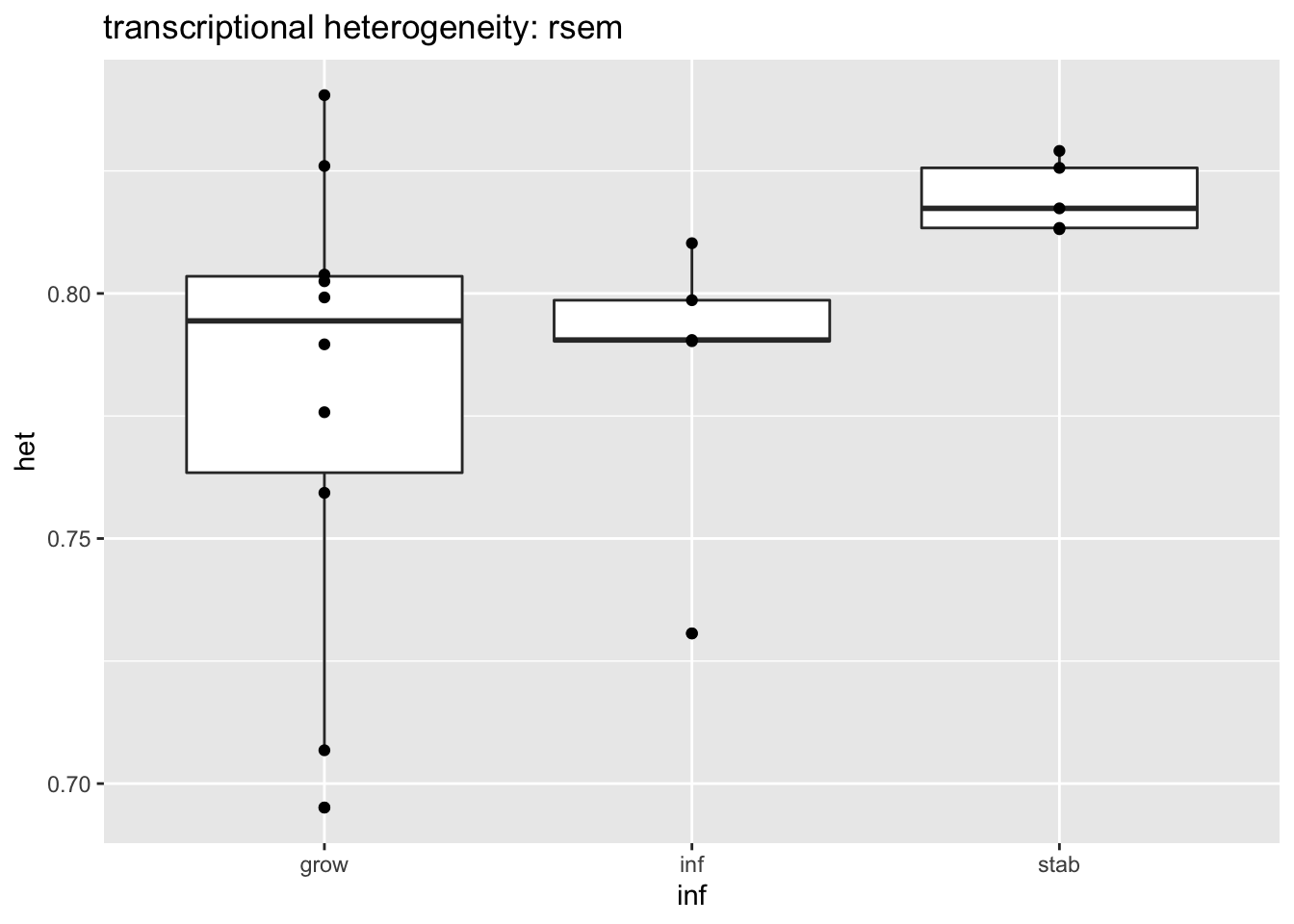
Figure 14.7: Transcriptional heterogeneity
wilcox.test(tab2$het[tab2$inf!="inf"]~tab2$inf[tab2$inf!="inf"])
##
##  Wilcoxon rank sum exact test
##
## data:  tab2$het[tab2$inf != "inf"] by tab2$inf[tab2$inf != "inf"]
## W = 9, p-value = 0.05528
## alternative hypothesis: true location shift is not equal to 0

write.csv(tab2, file="nature-tables/Ext5j_transcriptional_heterigeneity.csv")
14.5 Luminal-only non-inflammtory samples samples
We removed all the basal samples and did the same comparison:
Epdds$HR=Cdata$HR_status[match(substr(colnames(Epdds), 1, nchar(colnames(Epdds))-3), Cdata$TumorID)]
vstLumOnly=Epdds[, which(Epdds$HR=="Lum")]
design(vstLumOnly)=~Growth
vstLumOnly=DESeq(vstLumOnly)
colnames(Epdds)
##  [1] "10L_D_Ep"  "10R_BL_Ep" "11L_B_Ep"  "11N_D_Ep"  "11R_D_Ep"  "11R_C_Ep"
##  [7] "12L_D_Ep"  "14N_C_Ep"  "14N_D_Ep"  "14R_B_Ep"  "15N_C_Ep"  "16L_C_Ep"
## [13] "17N_D_Ep"  "2N__Ep"    "3N_B_Ep"   "3R_C_Ep"   "6R_B_Ep"   "7N_A_Ep"
## [19] "8L_D_Ep"   "8R_CU_Ep"

vstLumRes=results(vstLumOnly)
vsdLumvst=vst(vstLumOnly)

write.csv(vstLumRes, file="nature-tables/5j_lumonly_ep_growing_vs_stable.csv")
genes2=rownames(vstLumRes)[which(vstLumRes$padj<0.05 & abs(vstLumRes$log2FoldChange)>1.5 & vstLumRes$baseMean>100)]

GlistGrowing=rownames(vstLumRes)[which(vstLumRes$padj<0.05 & (vstLumRes$log2FoldChange)<(-1.5) & vstLumRes$baseMean>100)]
Glistnon=rownames(vstLumRes)[which(vstLumRes$padj<0.05 & (vstLumRes$log2FoldChange)>(1.5) & vstLumRes$baseMean>100)]
write.csv(GlistGrowing,file="figure-outputs/lumsig_posFC.csv" )
write.csv(Glistnon,file="figure-outputs/lumsig_negFC.csv" )

ColSideCols=ColSizeb[vstLumOnly$Growth]
#pdf("figure-outputs/Figure5_XX_heatmap_lumonly_growing_vs_stable.pdf", height=9, width=5)

heatmap.2(assay(vsdLumvst)[ genes2,  ], scale="row", trace="none", ColSideColors = brewer.pal(3, "Greens")[ColSideCols], col=RdBu[11:1], main="Ep genes" )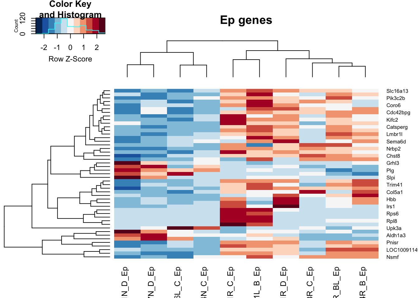
Figure 14.8: DEG non-inflamm Lum only
#dev.off()

#write.csv(assay(vsdLumvst)[ genes2,  ], file="nature-tables/5xx_lum_only_growing_vs_stable.csv")
#DT::datatable(as.data.frame(vstLumRes), rownames=F, class='cell-border stripe',
#          extensions="Buttons", options=list(dom="Bfrtip", buttons=c('csv', 'excel')))
Quickly run GSEA for these samples:
EpGenes=rownames(vstLumRes)

l1=SymHum2Rat$HGNC.symbol[match(EpGenes, SymHum2Rat$RGD.symbol)]
l2=Rat2Hum$HGNC.symbol[match(EpGenes, Rat2Hum$RGD.symbol)]
l3=Mouse2Hum$HGNC.symbol[match(EpGenes, Mouse2Hum$MGI.symbol)]
EpGenesConv=ifelse(is.na(l1)==F, l1, ifelse(is.na(l2)==F, l2, ifelse(is.na(l3)==F, l3, EpGenes)))


hits=EpGenesConv[match(rownames(vstLumRes), EpGenes)]
fcTab=vstLumRes$log2FoldChange
names(fcTab)=EpGenesConv


  gscaepNI_lum=GSCA(listOfGeneSetCollections=ListGSC,geneList=fcTab, hits = hits)
  gscaepNI_lum<- preprocess(gscaepNI_lum, species="Hs", initialIDs="SYMBOL",
                    keepMultipleMappings=TRUE, duplicateRemoverMethod="max",
                    orderAbsValue=FALSE)
## -Preprocessing for input gene list and hit list ...
## --Removing genes without values in geneList ...
## --Removing duplicated genes ...
## --Converting annotations ...
## -- 527 genes (out of 12341) could not be mapped to any identifier, and were removed from the data.
## -- 527 genes (out of 12341) could not be mapped to any identifier, and were removed from the data.
## --Ordering Gene List decreasingly ...
## -Preprocessing complete!
  gscaepNI_lum <- analyze(gscaepNI_lum,
                 para=list(pValueCutoff=0.05, pAdjustMethod="BH",
                           nPermutations=100, minGeneSetSize=5,
                           exponent=1),
                           doGSOA = F)
## --146 gene sets don't have >= 5 overlapped genes with universe in gene set collection named c2List!
## --848 gene sets don't have >= 5 overlapped genes with universe in gene set collection named c5BP!
## --269 gene sets don't have >= 5 overlapped genes with universe in gene set collection named c5MF!
## --110 gene sets don't have >= 5 overlapped genes with universe in gene set collection named c5CC!
## --377 gene sets don't have >= 5 overlapped genes with universe in gene set collection named MetPathway!
## -Performing gene set enrichment analysis using HTSanalyzeR2...
## --Calculating the permutations ...
## -Gene set enrichment analysis using HTSanalyzeR2 complete
## ==============================================

A1=HTSanalyzeR2::summarize(gscaepNI_lum)
##
## -No of genes in Gene set collections:
##                 input above min size
## c2List           2199           2053
## c5BP             7530           6682
## c5MF             1663           1394
## c5CC              999            889
## ProcessNetworks   158            158
## MetPathway       1480           1103
## Hallmark           50             50
##
##
## -No of genes in Gene List:
##           input valid duplicate removed converted to entrez
## Gene List 12449 12449             12341               11814
##
##
## -No of hits:
##      input preprocessed
## Hits 12449        11814
##
##
## -Parameters for analysis:
##               minGeneSetSize pValueCutoff pAdjustMethod
## HyperGeo Test 5              0.05         BH
##
##      minGeneSetSize pValueCutoff pAdjustMethod nPermutations exponent
## GSEA 5              0.05         BH            100           1
##
##
## -Significant gene sets (adjusted p-value< 0.05 ):
##          c2List c5BP c5MF c5CC ProcessNetworks MetPathway Hallmark
## HyperGeo     NA   NA   NA   NA              NA         NA       NA
## GSEA        243  768   98  100              52         84       22
## Both         NA   NA   NA   NA              NA         NA       NA

PNresultsef=gscaepNI_lum@result$GSEA.results$ProcessNetworks

TermsA=sapply(strsplit(rownames(gscaepNI_lum@result$GSEA.results$ProcessNetworks), "_"), function(x) x[2])
TermsA[which(is.na(TermsA))]=substr(rownames(gscaepNI_lum@result$GSEA.results$ProcessNetworks)[which(is.na(TermsA))], 2, 50)

save(gscaepNI_lum, file="figure-outputs/5xx_lumonly.Rdata") # save this file to change the colors

## check whether this runs:
gscaepNI_lum@result$GSEA.results$ProcessNetworks$Gene.Set.Term=TermsA
viewEnrichMap(gscaepNI_lum, gscs=c("ProcessNetworks"),
              allSig = TRUE, gsNameType="term" )
Figure 14.9: luminal non inflammatory branch
Repeat the above analysis performing leave one out
SigList=list()

for (i in 1:10){
vstLumOnly2=DESeq(vstLumOnly[ ,-i])
vstLumRes=results(vstLumOnly2)
genes3=rownames(vstLumRes)[which(vstLumRes$padj<0.05 & abs(vstLumRes$log2FoldChange)>1.5 & vstLumRes$baseMean>100)]
SigList[[i]]=genes3
}

## Collapse the results together and see how frequently each gene appears

N2=table(unlist(SigList))

Bx=names(N2)%in%c(GlistGrowing, Glistnon)
N2tab=data.frame(gene=names(N2), LOODEG=N2, InOrigList=Bx)

write.csv(N2tab, file="figure-outputs/5j_lumonly_ep_growing_vs_stable_LOO_analysis.csv")