Chapter 26 CNV calling
CNV calling was performed with BICseq
26.1 Sample data
Load BICseq2 data for all tested samples:
allfiles=dir("../data/CNV_calls/","2_scale$", full.names = T)

CNVL2=lapply(allfiles, function(x) read.delim(x, stringsAsFactors = F))
names(CNVL2)=unlist(sapply(strsplit(allfiles, "//|_cnv"), function(x) x[2]))
meltCN=melt(CNVL2, measure.vars=c("log2.copyRatio"))

AllDCN=data.frame(sampleID=meltCN$L1, chrom=substr(meltCN$chrom, 4, 5), start.pos=meltCN$start,
                   end.pos=meltCN$end, n.probes=meltCN$binNum, mean=meltCN$value,
                   call=ifelse(meltCN$value>0.3, "+", ifelse(meltCN$value<(-0.3), "-", "0")))

AllDCN2=data.frame(sample=meltCN$L1, chromosome=meltCN$chrom, start=meltCN$start,
                  end=meltCN$end, n.probes=meltCN$binNum, segmean=2*2^(meltCN$value),
                  call=ifelse(meltCN$value>0.3, "+", ifelse(meltCN$value<(-0.3), "-", "0")))

AllDCN2$chromosome=factor(AllDCN2$chromosome, levels=unique(AllDCN2$chromosome))

#CNVGRanges=GRanges(seqnames = AllDCN$chrom, ranges=IRanges(start=AllDCN$start.pos, end=AllDCN$end.pos), copy_ratio=AllDCN$mean, call=AllDCN$call, sample=AllDCN2$sample)

CNVGRanges=GRanges(seqnames = AllDCN2$chromosome, ranges=IRanges(start=AllDCN2$start, end=AllDCN2$end), segmean=AllDCN2$segmean, call=AllDCN2$call, sample=AllDCN2$sample)
26.2 Data Summary
26.2.1 Frequency of gains and losses across the genome
# plot the frequencies
Samp1=cnFreq_mod(AllDCN2,CN_low_cutoff=1.4, CN_high_cutoff=2.8, genome=cytoInfo)
Samp1$plot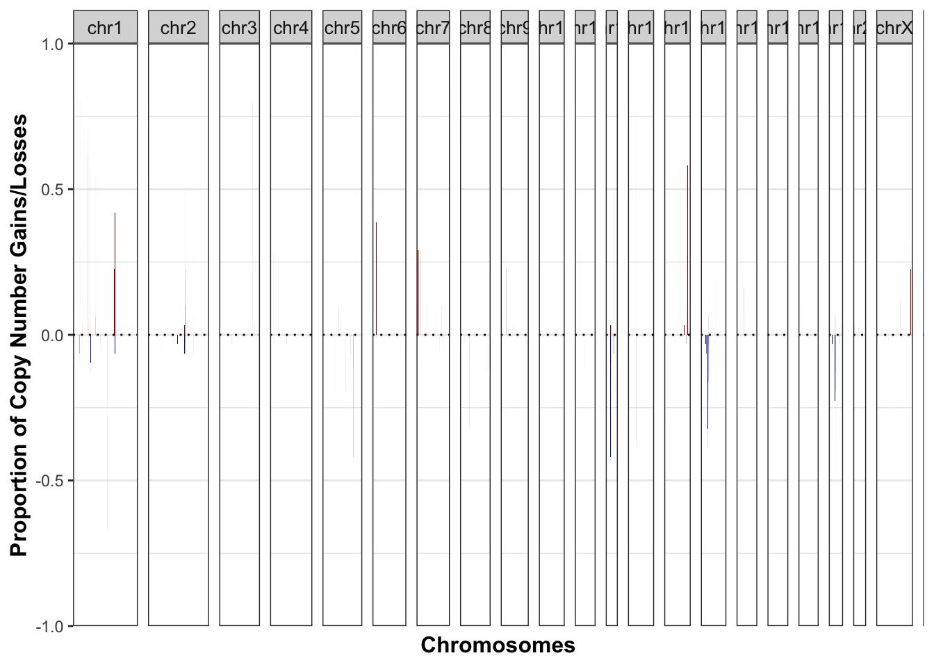
Figure 26.1: summary of regions of frequent gains and losses
26.2.2 Loci which have a hit in at least 30% of samples
# Filter out gain and loss regions
LocationsA=Samp1$data[which(Samp1$data$gainProportion>0.3), ]
LocationsA=LocationsA[order( LocationsA$chromosome, LocationsA$start),  ]
LocAmerge=Merge_contig(LocationsA)

LocationsB=Samp1$data[which(Samp1$data$lossProportion>0.3), ]
LocationsB=LocationsB[order( LocationsB$chromosome, LocationsB$start),  ]
LocBmerge=Merge_contig(LocationsB)

# turn into a GRanges object

LocAGRanges=GRanges(seqnames = LocAmerge$chromosome, ranges=IRanges(start=LocAmerge$start, end=LocAmerge$end), strand="*",
                    sampleFrequency=LocAmerge$sampleFrequency, gainFrequency=LocAmerge$gainFrequency, lossFrequency=LocAmerge$lossFrequency, gainProportion=LocAmerge$gainProportion, lossProportion=LocAmerge$lossProportion)

LocBGRanges=GRanges(seqnames = LocBmerge$chromosome, ranges=IRanges(start=LocBmerge$start, end=LocBmerge$end), strand="*",
                    sampleFrequency=LocBmerge$sampleFrequency, gainFrequency=LocBmerge$gainFrequency, lossFrequency=LocBmerge$lossFrequency, gainProportion=LocBmerge$gainProportion, lossProportion=LocBmerge$lossProportion)

# find the overlaps
GainOLap=findOverlaps(LocAGRanges, txRn6)
UniqueGainOlapRegions=unique(queryHits(GainOLap))
GainGenes=sapply(unique(queryHits(GainOLap)), function(x) txRn6$gene_id[subjectHits(GainOLap[which(queryHits(GainOLap)==x)])])

LossOLap=findOverlaps(LocBGRanges, txRn6)
UniqueLossOlapRegions=unique(queryHits(LossOLap))
LossGenes=sapply(unique(queryHits(LossOLap)), function(x) txRn6$gene_id[subjectHits(LossOLap[which(queryHits(LossOLap)==x)])])
Venn diagrams of the number of genes which intersect with the cosmic dataset
OverviewG=unique(unlist(GainGenes))
OverviewL=unique(unlist(LossGenes))

par(mfrow=c(1,2))
venn(list(CNVgains=OverviewG, cosmic=RatCosmic))
venn(list(CNVloss=OverviewL, cosmic=RatCosmic))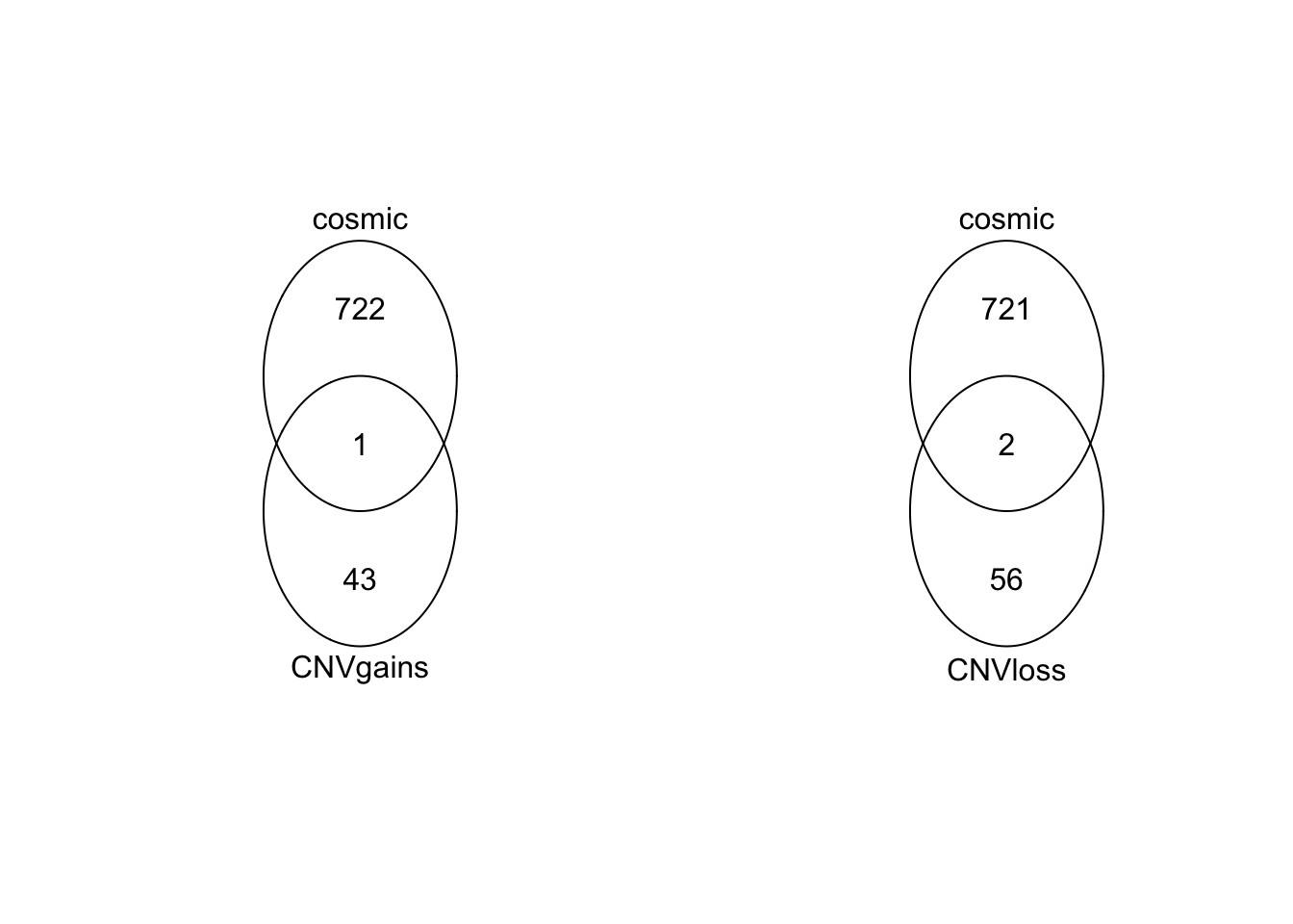
The intersecting gene is Lrp1b, Grin2a
Venn diagram of immune related genes:
par(mfrow=c(1,2))
venn(list(CNVgains=OverviewG, Immune=RatAllImm))
venn(list(CNVloss=OverviewL, Immune=RatAllImm))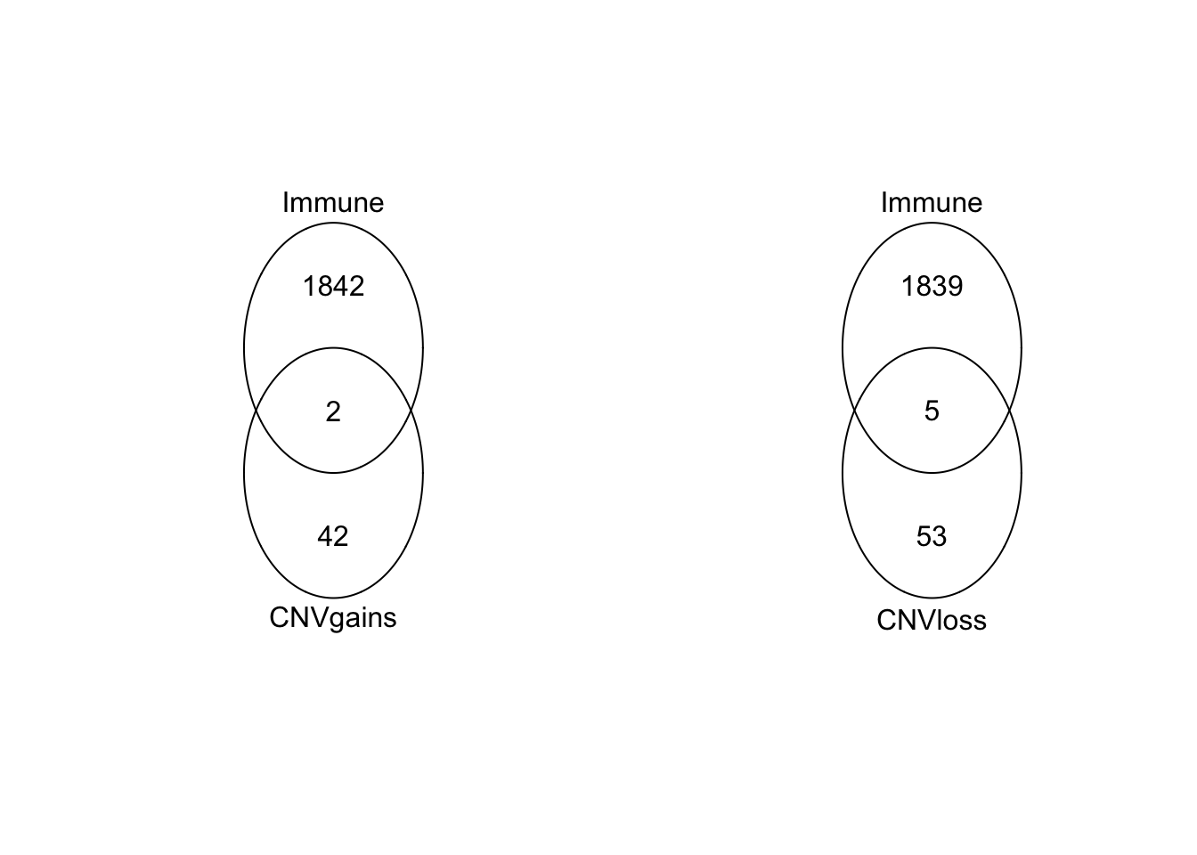
The gained genes are Mir295-2, Scarb1 The lost genes are Ccl28, Mff, Pdcd1, Arrb2, Mx2
26.2.3 Annotated plot of genome and locations of genes
S2=Samp1$data
S2=S2[order(S2$chromosome, S2$start), ]


GG2=sapply(GainGenes, length)
GG3=unlist(GainGenes)
GG3[which(duplicated(GG3))]=""
GG4=split(GG3, rep(c(1:length(GG2)), times=GG2))
Ggenes=sapply(GG4, function(x) paste(x, sep="", collapse=" "))
Ggenes=gsub("  ", "", Ggenes)
Ggenes[which(Ggenes==" ")]=""
Datx=rep("", nrow(Samp1$data))
Datx[match(LocAmerge$start[UniqueGainOlapRegions], S2$start)]=Ggenes

GG2=sapply(LossGenes, length)
GG3=unlist(LossGenes)
GG3[which(duplicated(GG3))]=""
GG4=split(GG3, rep(c(1:length(GG2)), times=GG2))
Lgenes=sapply(GG4, function(x) paste(x, sep="", collapse=" "))
Lgenes[which(Lgenes==" ")]=""
Daty=rep("", nrow(Samp1$data))
Daty[match(LocBmerge$start[UniqueLossOlapRegions], S2$start)]=Lgenes

##
#S2=Samp1$data
#S2=S2[order(S2$chromosome, S2$start), ]
S2$xLoc=S2$start+chrInfo$sumdist[match(S2$chromosome, chrInfo$Chromosome)]
S2$width=S2$end-S2$start
S2$label=Datx

S3=S2
S3$gainProportion=S3$lossProportion[1:nrow(S2)]*(-1)
S3$label=Daty

S4=rbind(cbind(S3, col="blue"), cbind(S2, col="red"))
S4=S4[-which(S3$gainProportion==0), ]

ggplot(S4, aes(x=xLoc, y=gainProportion, width=width*1.2, label=label, col=col))+geom_bar(stat = "identity")+geom_label_repel()+theme_bw()+xlim(0, chrInfo$sumdist2[22])+geom_vline(xintercept=chrInfo$sumdist2,col="grey")+scale_colour_manual(values=c("blue", "red"))+annotate("text", x=chrInfo$sumdist, y=rep(-1, 22), label=chrInfo$Chromosome, col="black")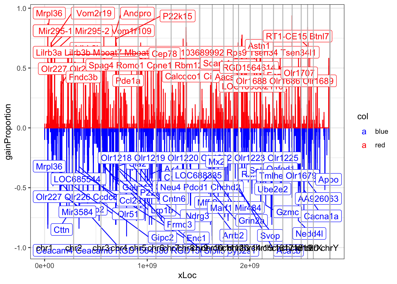
26.3 Samples with CNVs in breast-related genes
Below is the plot showing the breast-related mutations as well as CNVs added
ttemp=CNVGRanges[which(CNVGRanges$call!=0)]
Bsamples=txRn6[which(txRn6$gene_id%in%c(RatBreastCosmic, OtherBreast))]
olaps=findOverlaps(Bsamples,ttemp)
ttemp$gene=NA
ttemp$gene[subjectHits(olaps)]=Bsamples$gene_id[queryHits(olaps)]
ttemp$NewID=sapply(ttemp$sample, function(x) Cdata$NewID[grep(x, Cdata$WGS)])

x1=which(!is.na(ttemp$gene))
l1=match(ttemp$gene[x1], colnames(X2b))
lnew=unique(ttemp$gene[x1[which(is.na(l1))]])
X2b=cbind(X2b, matrix(0, ncol=length(lnew), nrow=nrow(X2b)))
colnames(X2b)[(ncol(X2b)-length(lnew)+1):ncol(X2b)]=lnew
l1=match(ttemp$gene[x1], colnames(X2b))
l2=match(ttemp$NewID[x1], rownames(X2b))
for (i in 1:length(l1)){
  X2b[l2[i],l1[i]]=ifelse(ttemp$call[x1[i]]=="+", 5, 4)
}
l2=rowSums(sign(X2b))
l3=colSums(sign(X2b))
heatmap.2(X2b[order(l2),order(l3) ], col=c("white",  3:5, 2:1), scale="none", trace="none", sepcolor="grey85", colsep=c(1:ncol(X2b)), rowsep=c(1:nrow(X2b)), sepwidth=c(0.005, 0.005))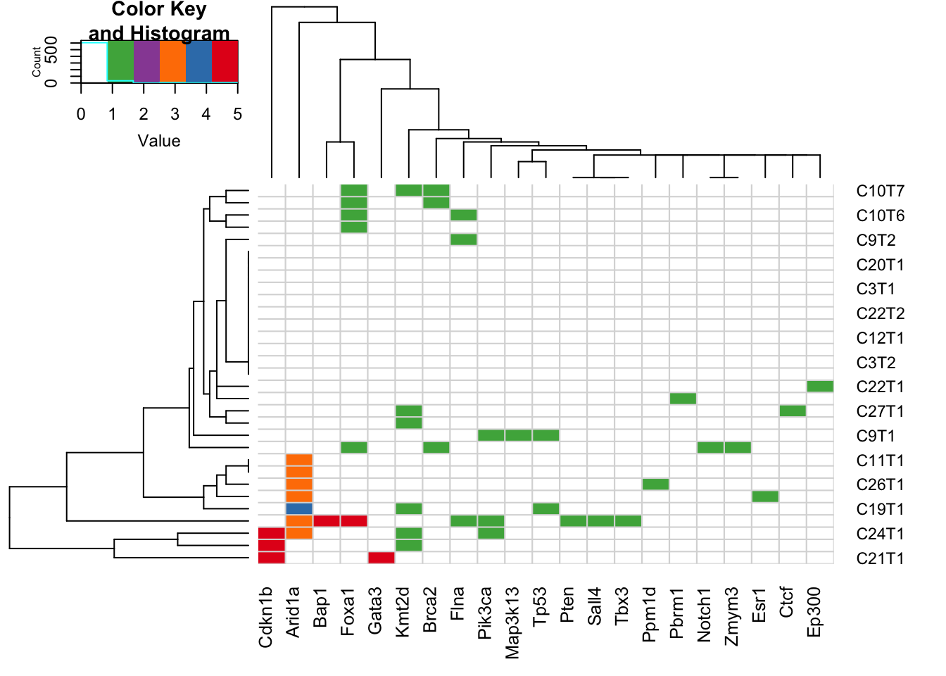
Matching the frequency data with genes
S1GR=GRanges(seqnames = Samp1$data$chromosome, ranges=IRanges(start=Samp1$data$start, end=Samp1$data$end))
olaps=findOverlaps(S1GR, txRn6)
Samp1$data$gene=NA
Samp1$data$gene[queryHits(olaps)]=txRn6$gene_id[subjectHits(olaps)]

gid=unique(na.omit(Samp1$data$gene))
Tabix=matrix(0, nrow=length(gid), ncol=2)
rownames(Tabix)=gid

for (i in gid){
  m1=Samp1$data[which(Samp1$data$gene==i), ]
  Tabix[i, ]=colMedians(data.matrix(m1[ , 7:8]))

}


rownames(Tabix)=toupper(rownames(Tabix))

Tabix=Tabix[order(rownames(Tabix)), ]
Tabix=Tabix[-which(rowSums(Tabix)==0), ]

lx=match( names(rGene2), rownames(Tabix))

df2=data.frame(mut=rGene2, gain=Tabix[ lx,1], loss=Tabix[lx, 2])

lx2=match(rownames(Tabix), names(rGene2))

df3=data.frame(mut=0, gain=Tabix[which(is.na(lx2)),1], loss=Tabix[which(is.na(lx2)),2])

dfAll=rbind(df2, df3)

#mx=which(rownames(dfAll)%in%AllCosmic$Gene.Symbol)
dfAll[which(is.na(dfAll), arr.ind=T)]=0
dfAll=dfAll*100
dfAll[ ,3]=dfAll[ ,3]*(-1)
dfAll$gene=rownames(dfAll)

dfAll=dfAll[ ,c(4, 1:3)]
mx=which(dfAll$gene%in%AllCosmic$Gene.Symbol)
write.table(dfAll[mx, ], file="nature-tables/outputs_pathway_map_cosmic.txt", quote = F, row.names = F, sep="\t")
26.4 Summary of the sequencing depth
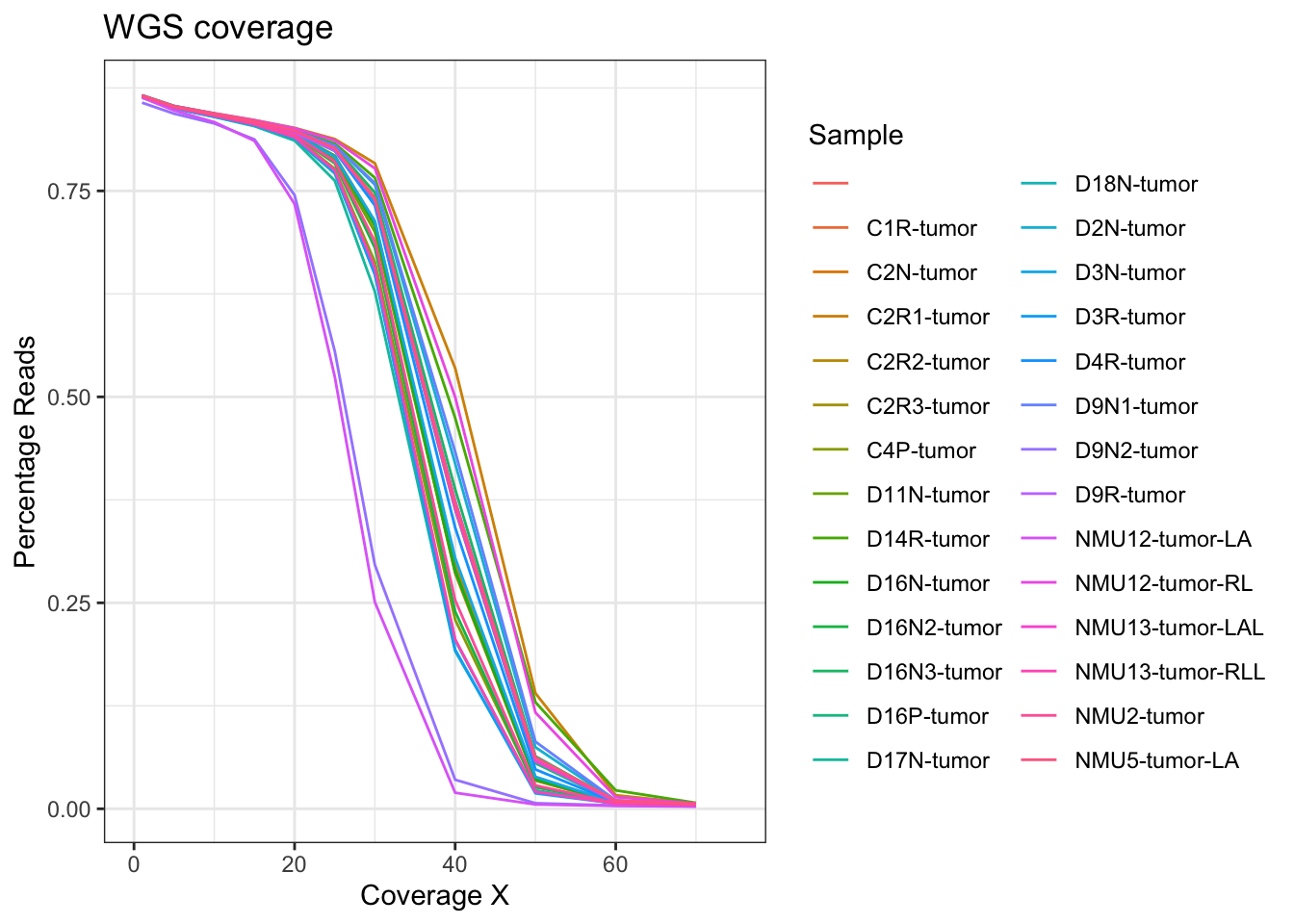
Below, do a quick summary of the WGS data: what is the coverage, and plot the percentage mapping of the coverage:
SeqData=read.delim("../data/wholegenome_mutations/summary_Sequencing_output.txt", sep="\t")

hist(SeqData$MEAN_COVERAGE, breaks=10)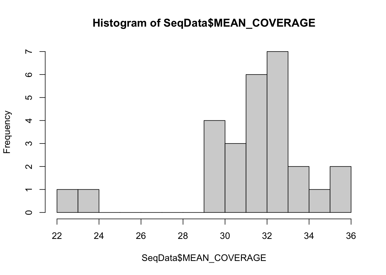
Also, extract the information about coverage:
SeqDatam=melt(SeqData[ ,c(grep("PCT_[0-9]*X", colnames(SeqData)), ncol(SeqData))])
SeqDatam$coverage2=sapply(strsplit(as.character(SeqDatam$variable), "_"), function(x) x[2])
SeqDatam$coverage3=as.numeric(substr(SeqDatam$coverage2, 1, nchar(SeqDatam$coverage2)-1))


ggplot(SeqDatam, aes(x=coverage3, y=value, col=Sample))+geom_line()+theme_bw()+ggtitle("WGS coverage")+ylab("Percentage Reads")+xlab("Coverage X")+xlim(c(0, 75))