Chapter 25 Trichrome staining
Quantification of trichrome staining was performed in Qupath using the following steps:
- image is loaded as a “DAB” image
- using “gold standard” trichrome-stained images with good stroma and epithelial content, estimate the stain vectors
- Perform color deconvolution
- A pixel classifier was used to estimate trichrome content
- A pixel classifier was used to estimate tumor content
A snippet of the qupath script is shown below:
# insert some text here

setImageType('BRIGHTFIELD_H_DAB');
setColorDeconvolutionStains('{"Name" : "trichrome", "Stain 1" : "Hematoxylin", "Values 1" : "0.71695 0.66336 0.21432 ", "Stain 2" : "DAB", "Values 2" : "0.46299 0.76212 0.45257 ", "Background" : " 255 255 255 "}');
selectAnnotations();
addPixelClassifierMeasurements("stroma_classifier_again", "stroma_classifier_again")
selectAnnotations();
addPixelClassifierMeasurements("test_tumor", "test_tumor")

def entry = getProjectEntry()
def name = entry.getImageName() + '.txt'
def path = buildFilePath(PROJECT_BASE_DIR, 'annotation results')
mkdirs(path)
path = buildFilePath(path, name)
saveAnnotationMeasurements(path)
25.1 Associations with cellular fraction (wsi)
# load the data
TrichromeData=read.xlsx("../data/trichrome-staining-result.xls", 1)
midx=match(TrichromeData$SampleID, gsub("_", "", Cdata$TumorID))

Cdata$Trichrome=NA
Cdata$Trichrome[na.omit(midx)]=TrichromeData$Percentage.Stroma[which(!is.na(midx))]

t2=WSIvalFracs[, match(rownames(df.Spatial), colnames(WSIvalFracs))]

df.Spatial=cbind(df.Spatial, t(t2))


df.Spatial$Trichrome=NA
midx=match(TrichromeData$SampleID, rownames(df.Spatial))
df.Spatial$Trichrome[na.omit(midx)]=TrichromeData$Percentage.Stroma[-which(is.na(midx))]
# plot associations

n2=c("CD8", "EpCAM", "SMA", "Unclass", "EpCAM: SMA")

#pdf("~/Desktop/richrome-association-WSI-data-Calc2.pdf", width=6, height=5)

par(mfrow=c(2,3))
for (i in n2){
   a1=cor.test(df.Spatial$Trichrome, df.Spatial[ ,match(i, colnames(df.Spatial))], use="complete")
   n1=paste(i, "cor:", round(a1$estimate,1), "p:", round(a1$p.value,2))
   plot(df.Spatial$Trichrome, df.Spatial[ ,match(i, colnames(df.Spatial))], main=n1, xlab="Trichrome", ylab=i)
}

#dev.off()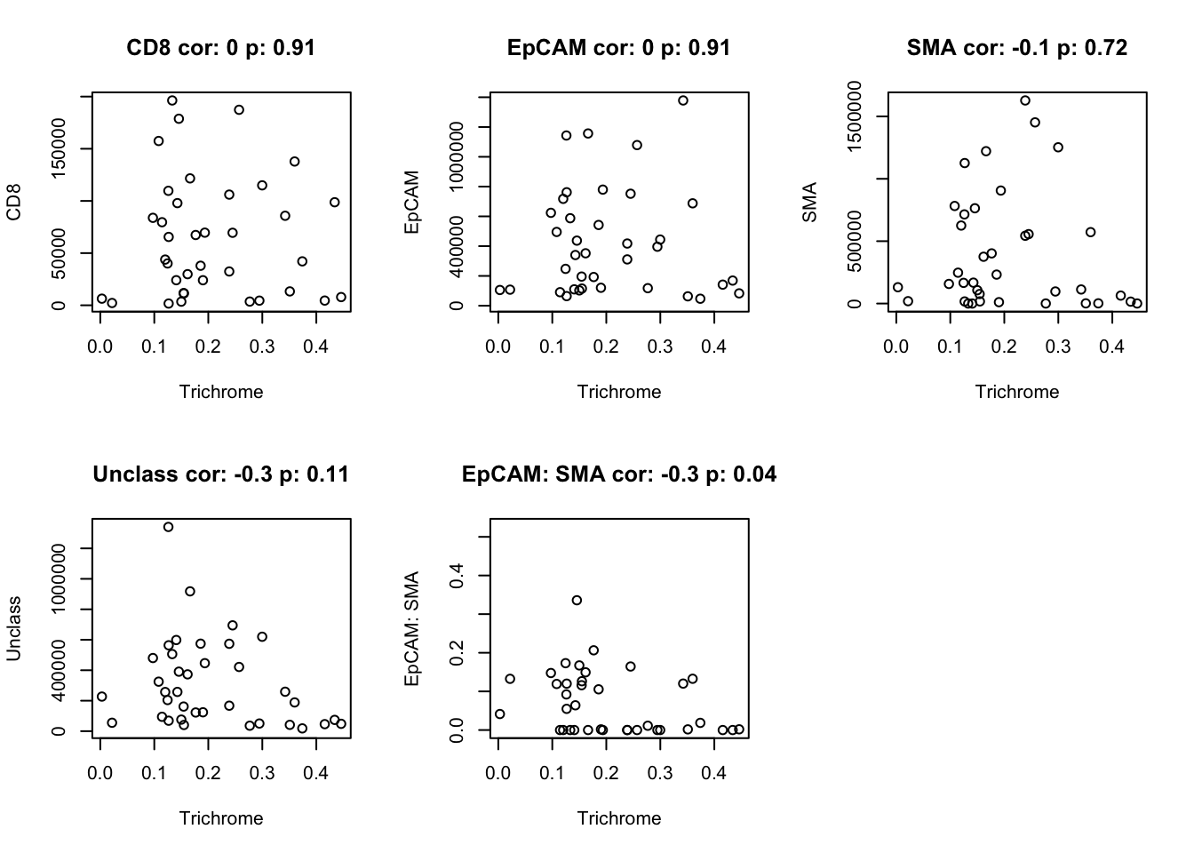
25.2 Associations with CD8 content
par(mfrow=c(1,2))

a1=wilcox.test(df.Spatial$Trichrome~df.Spatial$IF.EpCAMcut)$p.val
boxplot(df.Spatial$Trichrome~df.Spatial$IF.EpCAMcut, main=sprintf("Ep int. fraction %s", round(a1,2)))
a1=wilcox.test(df.Spatial$Trichrome~df.Spatial$CD8Fraccut)$p.val
boxplot(df.Spatial$Trichrome~df.Spatial$CD8Fraccut, main=sprintf("CD8 fraction vs Trichrome %s", round(a1,2)))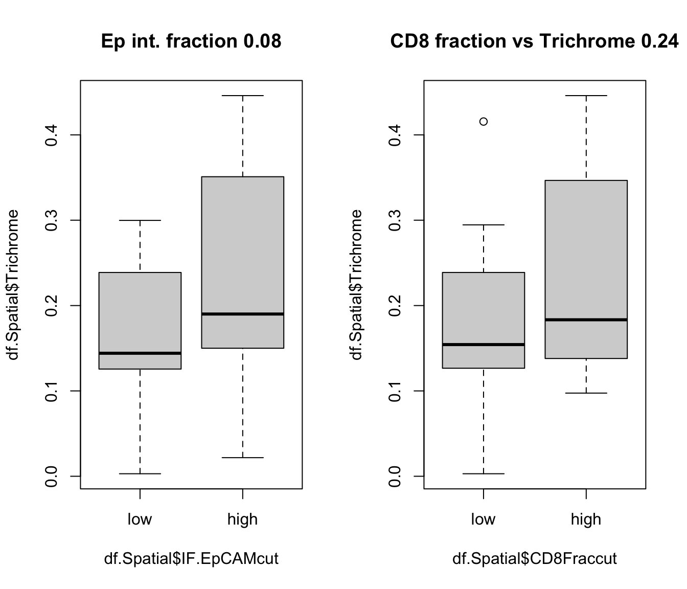
25.3 Associations with growth and treatment
df.Spatial$Growth=Cdata$Tumor.Growth[match(rownames(df.Spatial), gsub("_", "", Cdata$TumorID))]
df.Spatial$Treatment=Cdata$Treatment[match(rownames(df.Spatial), gsub("_", "", Cdata$TumorID))]
df.Spatial$NewID=Cdata$Treatment[match(rownames(df.Spatial), gsub("_", "", Cdata$NewID))]
df.Spatial$trichrome_pc=Cdata$Trichrome_encapsulation.[match(rownames(df.Spatial), gsub("_", "", Cdata$TumorID))]

pv1=sapply(c("PDL1", "LY", "PDL1+LY"), function(x) wilcox.test(df.Spatial$Trichrome[which(df.Spatial$Treatment%in%c("Vehicle", x))]~
           df.Spatial$Treatment[which(df.Spatial$Treatment%in%c("Vehicle", x))])$p.value)
names(pv1)=c("PDL1", "LY", "PDL1+LY")

ggplot(df.Spatial[ ,c("Treatment", "Trichrome")], aes(x=Treatment, y=Trichrome, col=Treatment))+geom_boxplot()+geom_jitter()+
scale_color_manual(values=ColMerge[ ,1])+theme_bw()+ggtitle(paste(paste(names(pv1), round(pv1, 2)), collapse=";"))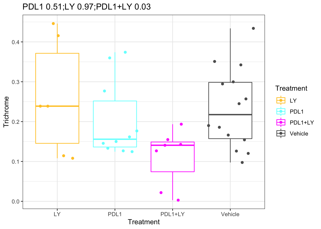
Figure 25.1: Trichrome staining with treatment
ggplot(df.Spatial[ ,c("Treatment", "trichrome_pc")], aes(x=Treatment, y=trichrome_pc, col=Treatment))+geom_boxplot()+geom_jitter()+
scale_color_manual(values=ColMerge[ ,1])+theme_bw()+ggtitle(paste(paste(names(pv1), round(pv1, 2)), collapse=";"))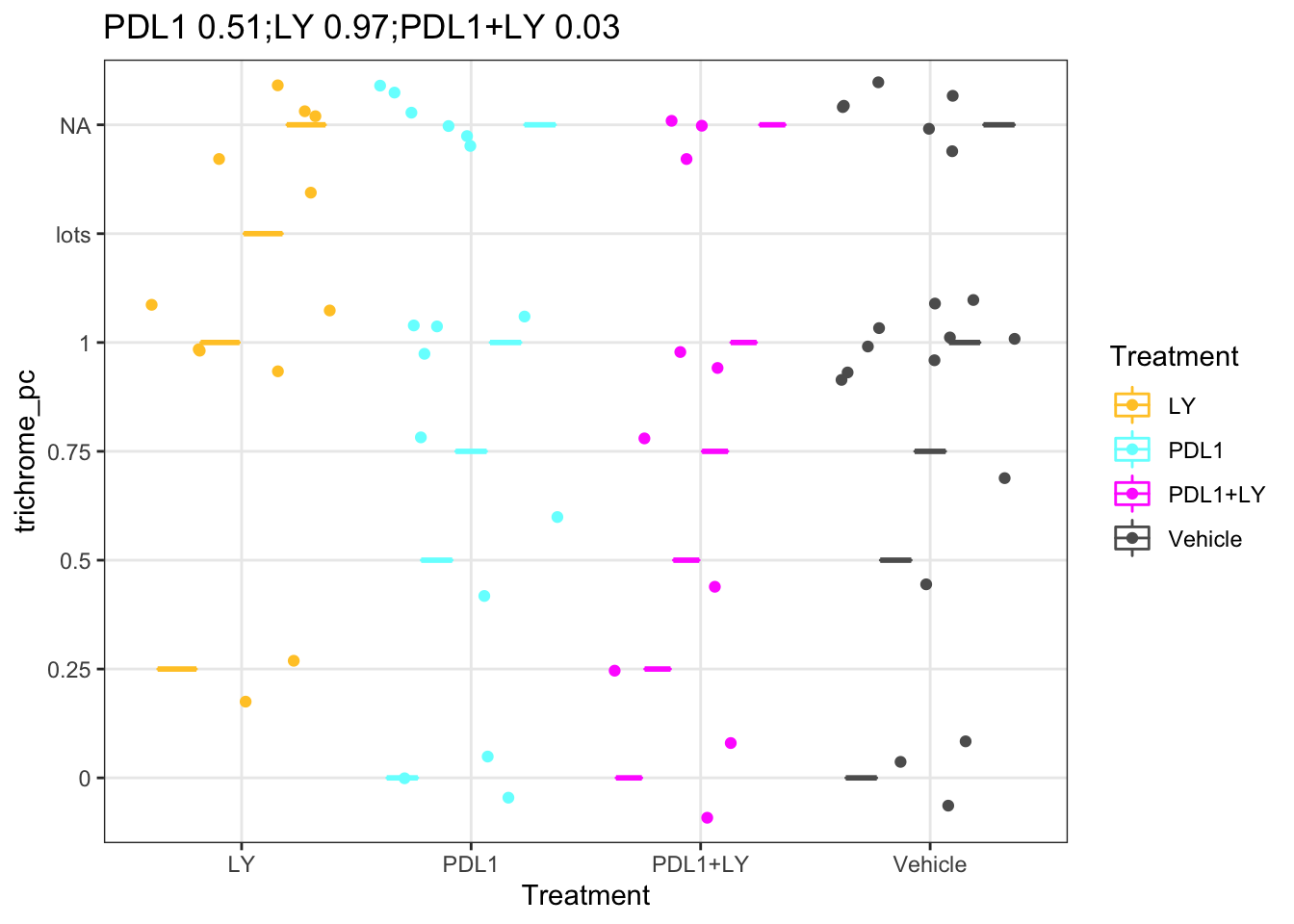
Figure 25.2: Trichrome staining with treatment
a1=df.Spatial[ ,match(c("Trichrome", "Growth", "trichrome_pc"), colnames(df.Spatial))]
a1a=wilcox.test(df.Spatial$Trichrome[which(df.Spatial$Growth=="growing")],
           df.Spatial$Trichrome[which(df.Spatial$Growth=="stable")])
a1a
##
##  Wilcoxon rank sum exact test
##
## data:  df.Spatial$Trichrome[which(df.Spatial$Growth == "growing")] and df.Spatial$Trichrome[which(df.Spatial$Growth == "stable")]
## W = 79, p-value = 0.04521
## alternative hypothesis: true location shift is not equal to 0

ggplot(a1, aes(x=Growth, y=Trichrome, col=Growth))+geom_boxplot()+geom_jitter()+
scale_color_manual(values=c(ColSize, "black"))+theme_bw()+ggtitle("growth") # round(a1a, 2)))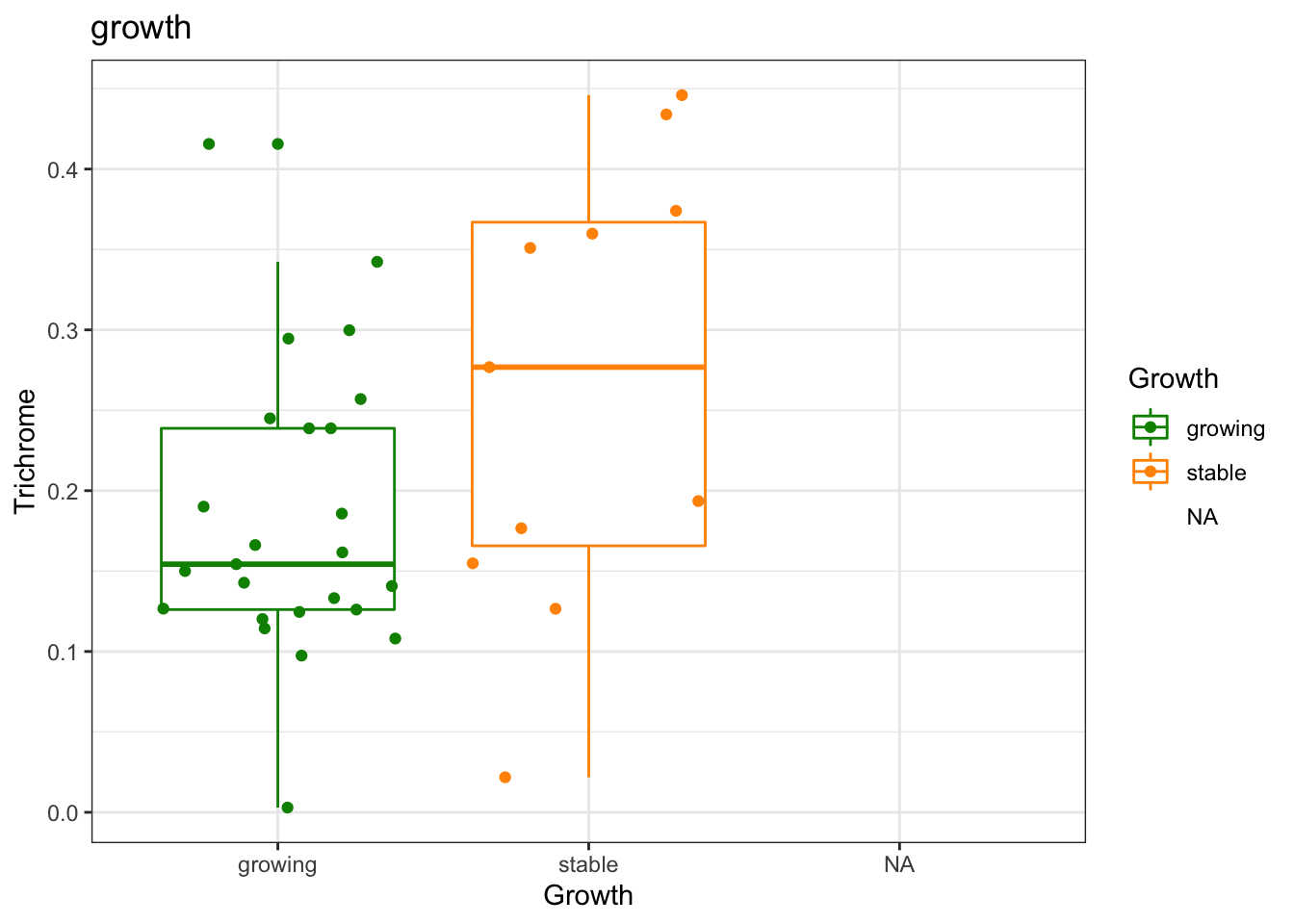
Figure 25.3: Trichrome with growth
ggplot(a1, aes(x=Growth, y=trichrome_pc, col=Growth))+geom_boxplot()+geom_jitter()+
scale_color_manual(values=c(ColSize, "black"))+theme_bw()+ggtitle("growth") # round(a1a, 2)))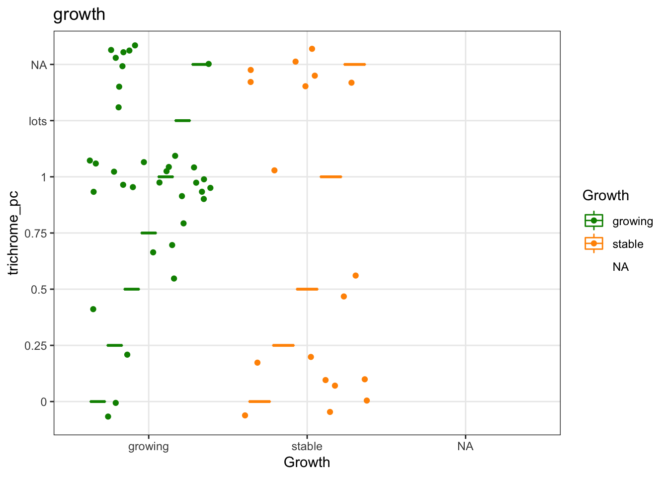
Figure 25.4: Trichrome with growth
#print(p)

#write.csv(df.Spatial[ ,c("Trichrome", "Growth", "Treatment")], file="nature-tables/3g_trichrome.csv")
DT::datatable(df.Spatial[ ,c("Trichrome", "Growth", "Treatment", "trichrome_pc")], rownames=F, class='cell-border stripe', extensions="Buttons", options=list(dom="Bfrtip", buttons=c('csv', 'excel'), scrollX=T))
Figure 25.5: Trichrome with growth
Trichrome encapsulation
df.Spatial$trichrome_pc[which(df.Spatial$trichrome_pc=="lots")]=1
df.Spatial$trichrome_pc[which(df.Spatial$trichrome_pc=="0% ignore")]=NA
df.Spatial$trichrome_pc
##  [1] "0.75" "0.5"  "0"    NA     NA     NA     "1"    NA     "1"    "0"
## [11] "1"    "1"    NA     "0"    "1"    "0.75" "0.25" "0"    "0"    NA
## [21] "0.5"  "1"    NA     NA     "1"    "0.5"  NA     "1"    "0"    "1"
## [31] "0.5"  "0.75" NA     "1"    "0"    "1"    "0"    "1"    "1"    NA
## [41] "1"    NA     NA     NA     NA     "1"    "1"    NA     "0.25" "1"
## [51] "1"    "1"    NA     NA     NA     "0.25" "1"    "1"
#wilcox.test(factor(as.numeric(df.Spatial$trichrome_pc))~df.Spatial$Growth)
25.4 Association with hyperinflammatory status
We can also do a boxplot for trichrome status and whether it associates with hyperinflammation in our rat samples
vstEpInf$Inflammation3
##  [1] inf  grow grow inf  grow grow grow grow grow grow grow grow grow grow inf
## [16] grow inf  grow inf  grow
## Levels: grow inf
vstEpInf$Inflammation2
##  [1] inf  grow grow inf  grow grow stab stab stab grow grow stab stab grow inf
## [16] grow inf  grow inf  grow
## Levels: grow inf stab
vstEpInf$Inflammation
##  [1] yes no  no  yes no  no  no  no  no  no  no  no  no  no  yes no  yes no  yes
## [20] no
## Levels: no yes
save(vstEpInf, file="figure-outputs/temp_test.RData")

ax1=colnames(vstEpInf)

t2=match(gsub("_", "", substr( ax1, 1, nchar(ax1)-2)), rownames(df.Spatial))

newTab=data.frame(trichrome=df.Spatial[na.omit(t2), "Trichrome"],
             inf=vstEpInf$Inflammation2[-which(is.na(t2))],
             names=ax1[-which(is.na(t2))],
             names2=rownames(df.Spatial)[na.omit(t2)])
wilcox.test(newTab$trichrome[newTab$inf=="grow"], newTab$trichrome[newTab$inf!="grow"])
##
##  Wilcoxon rank sum exact test
##
## data:  newTab$trichrome[newTab$inf == "grow"] and newTab$trichrome[newTab$inf != "grow"]
## W = 6, p-value = 0.04507
## alternative hypothesis: true location shift is not equal to 0
#pdf("figure-outputs/EXT5I_trichrome.pdf", height=5, width=4)
ggplot(newTab, aes(y=trichrome,x=inf))+geom_boxplot()+geom_point()+theme_bw()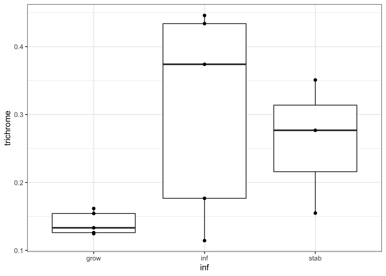
Figure 25.6: association with hyperinflammation
Also check the encapsulated status?
newTab$trichrome_pc=Cdata$Trichrome_encapsulation.[match(newTab$names2, gsub("_", "", Cdata$TumorID))]
newTab$trichrome_pc[which(newTab$trichrome_pc=="lots")]=1
newTab$trichrome_pc=as.numeric(newTab$trichrome_pc)
#pdf("figure-outputs/EXT5I_trichrome_pt2.pdf", height=5, width=4)
ggplot(newTab, aes(y=trichrome_pc,x=inf))+geom_boxplot()+geom_jitter(col="grey")+theme_bw()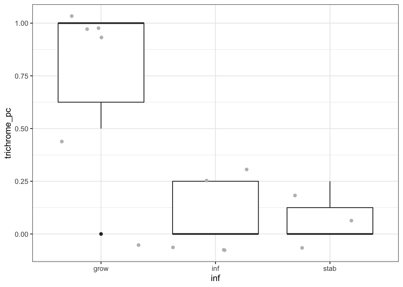
wilcox.test(newTab$trichrome_pc[newTab$inf=="grow"], newTab$trichrome_pc[newTab$inf!="grow"])
##
##  Wilcoxon rank sum test with continuity correction
##
## data:  newTab$trichrome_pc[newTab$inf == "grow"] and newTab$trichrome_pc[newTab$inf != "grow"]
## W = 42.5, p-value = 0.01389
## alternative hypothesis: true location shift is not equal to 0
DT::datatable(newTab, rownames=F, class='cell-border stripe',
          extensions="Buttons", options=list(dom="Bfrtip", buttons=c('csv', 'excel')))