Chapter 16 Read in ER i/o data
Read in data from cohort of samples which have ER
ERTPM=read.delim("../data/Tolaney/rnaseq_tpm_counts.txt", sep="\t", skip=1)
rownames(ERTPM)=ERTPM[ ,1]

ERcounts=read.delim("../data/Tolaney/raw_rnaseq_counts.txt", sep="\t")
ERcounts=ERcounts[-25800, ]
rownames(ERcounts)=ERcounts[ ,1]

ERClin=read.delim("../data/Tolaney/clin_data.txt", sep="\t", skip=1)

ERcibersort=read.csv("../data/Tolaney/CIBERSORT.csv", skip=1)
ERcytokines=read.csv("../data/Tolaney/cytokines.csv", skip=1)

## Append data where necessary:
ERClin$CD8_Tcell=ERcibersort$T.cells.CD8[match(paste("Patient", ERClin$Subject.ID, sep=""), ERcibersort$Patient)]
ERClin$DCs=ERcibersort$Dendritic.cells.activated[match(paste("Patient", ERClin$Subject.ID, sep=""), ERcibersort$Patient)]
ERClin$MICB=ERcytokines$MICB[match(ERClin$Subject.ID, ERcytokines$Subject.ID)]
ERClin$MICA=ERcytokines$MICA[match(ERClin$Subject.ID, ERcytokines$Subject.ID)]
There are 30 patients in this cohort
16.1 Signature: Lum cases non-inflammatory: growing vs stable
Here, use the signature which was applied before to see the difference between the non-inflammatory growing vs stable samples. We compare this to the oncotypedx list of genes and mammaprint
#GlistGrowing=read.csv("figure-outputs/lumsig_posFC.csv")
#GlistGrowing=GlistGrowing$x
#Glistnon=read.csv("figure-outputs/lumsig_negFC.csv")
#Glistnon=Glistnon$x
HumGeneList=SymHum2Rat$HGNC.symbol[match(GlistGrowing, SymHum2Rat$RGD.symbol)]
HumGeneList2=Rat2Hum$HGNC.symbol[match(GlistGrowing, Rat2Hum$RGD.symbol)]

TCGAssgsea=gsva(data.matrix(ERTPM[ ,-1]), list(grow=na.omit(HumGeneList2),  stab=Rat2Hum$HGNC.symbol[match(Glistnon, Rat2Hum$RGD.symbol)],Onco=Oncoprint[[1]], Mamma=Oncoprint[[2]]), method="ssgsea", ssgsea.norm=F)

TCGAssgsea=t(scale(t(TCGAssgsea)))

par(mfrow=c(1,2))
hist(TCGAssgsea[1, ], main="growing")
hist(TCGAssgsea[2, ], main="stable")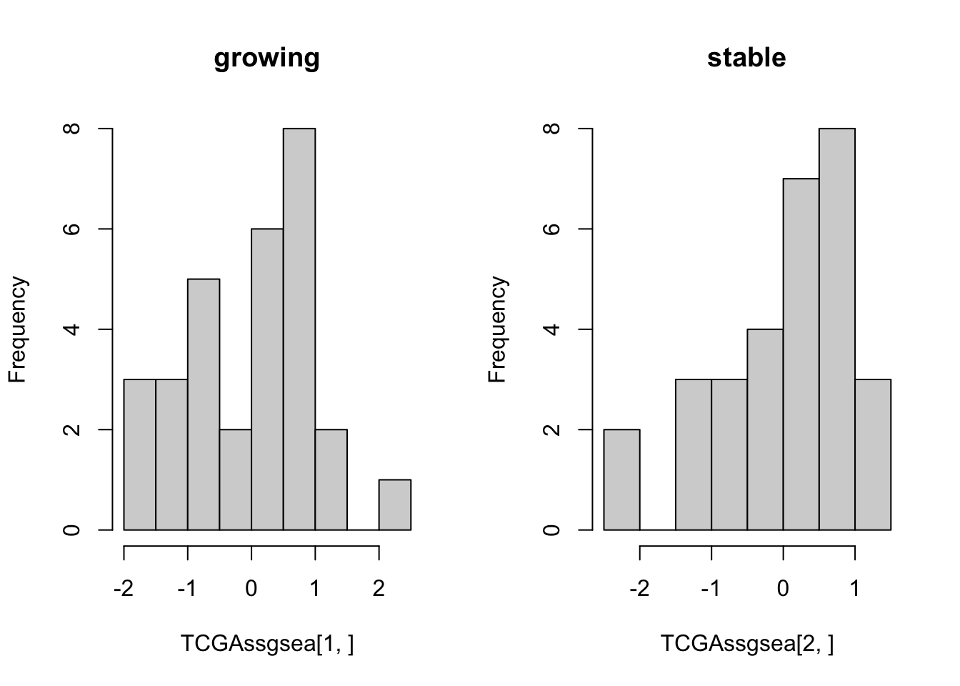
plot(TCGAssgsea[1, ], TCGAssgsea[2, ], ylab="stable", xlab="growing")

## also compare with onco or mamma print

plot(TCGAssgsea[1, ], TCGAssgsea[3, ], xlab="growing", ylab="oncotype")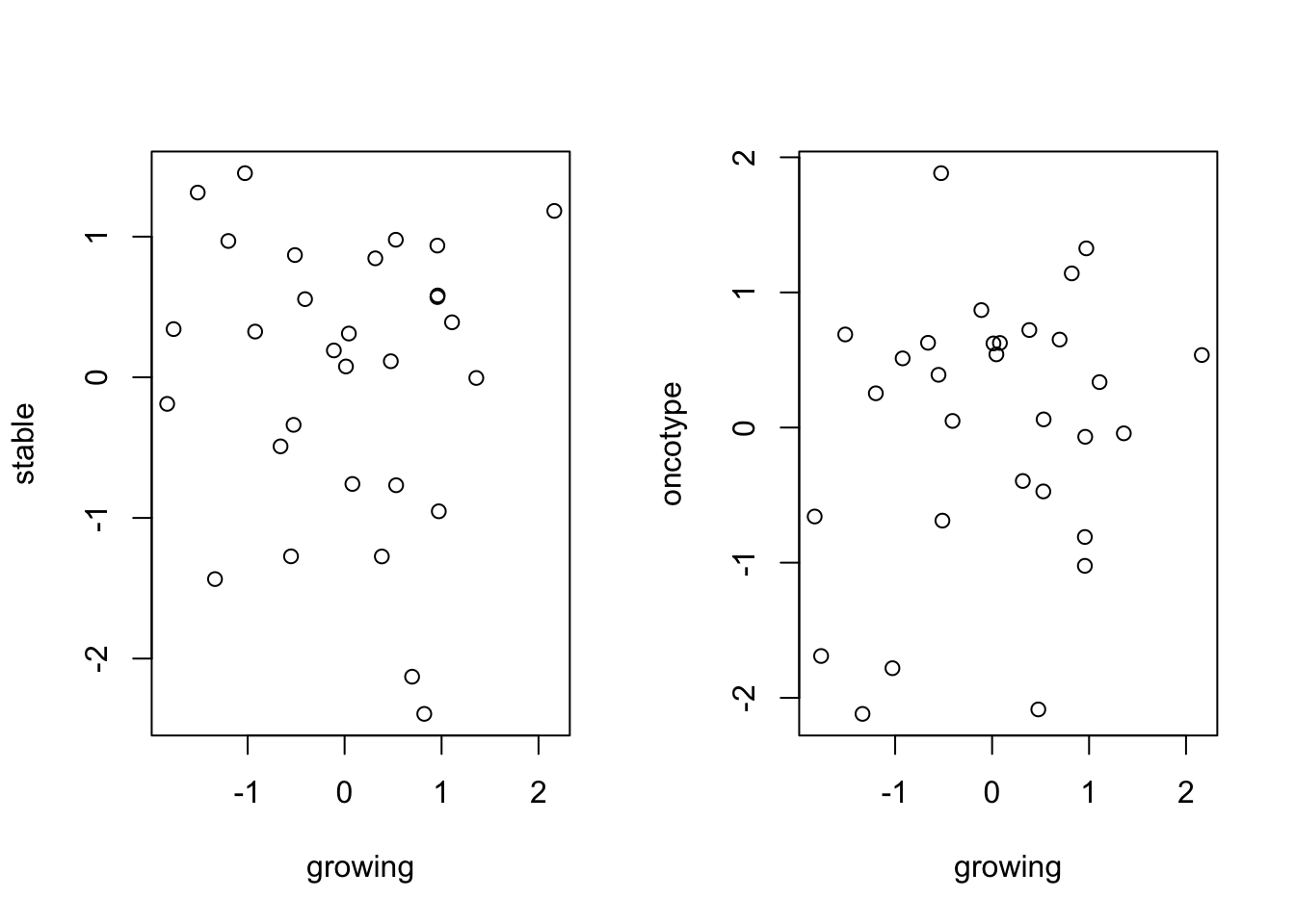
plot(TCGAssgsea[1, ], TCGAssgsea[4, ], xlab="growing", ylab="mammaprint")

## double check the

plot(TCGAssgsea[1, ], ERTPM["ADAMTS10" ,-1], xlab="growing sig", ylab="ADAMST10")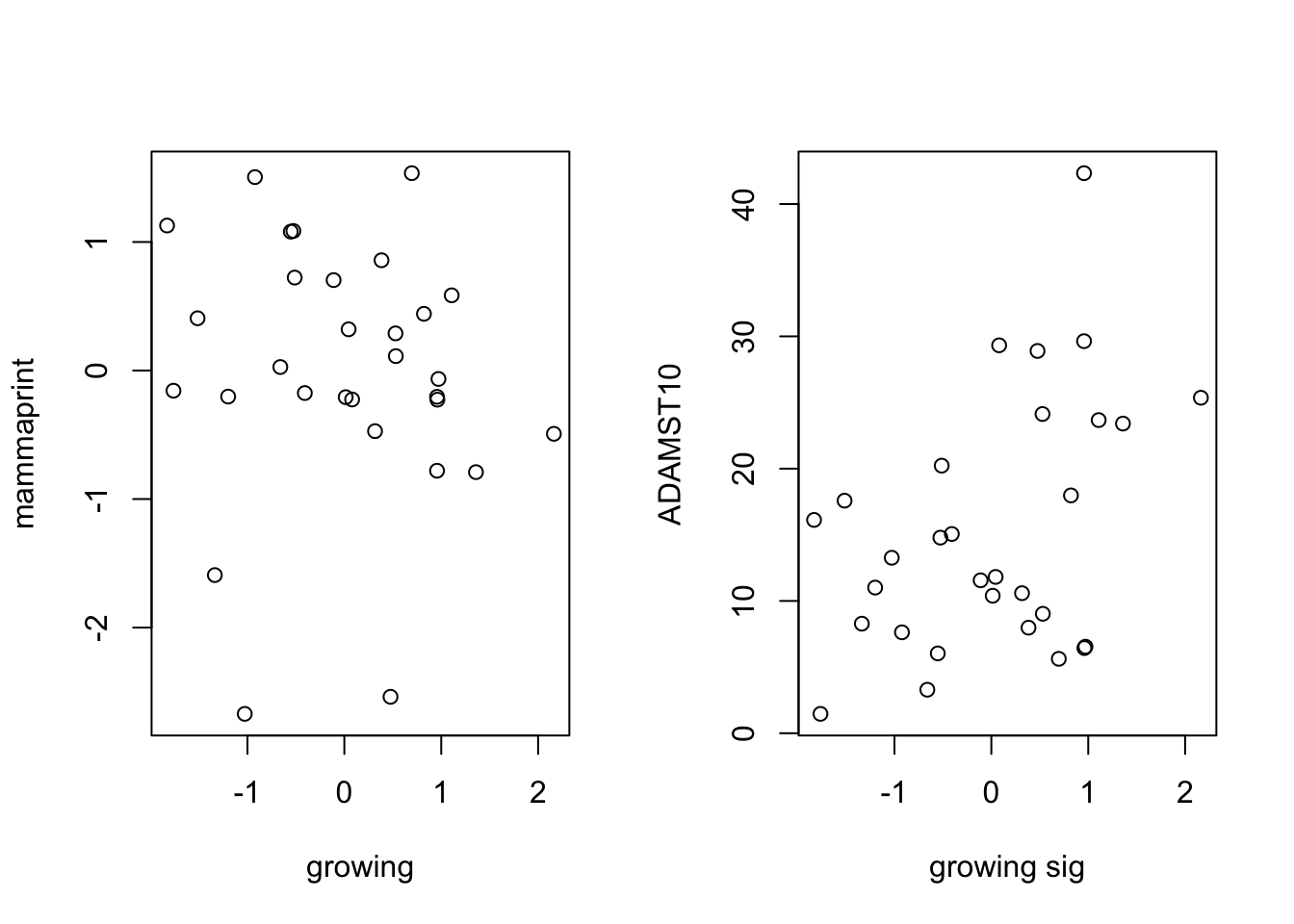
The Growing signature genes (positive coefficient) are Setd7, Hspa1l, Hbb, Kifc2, Kmt5c, Pik3c2b, Lmntd2, Nsmf, Nrbp2, LOC100134871, Hsp90aa1, Coro6, Chst8, Slc4a3, Fhod1, Rpl8, Spp1, Catsperg, Col5a1, LOC100911498, Noxa1, F8, Rps19, Rps6, Irs1, Leng8, Plekhh1, Lmbr1l, Ikbke, Pnisr, Adamts10, Zfp692, Trim41, Sema6d, Mgp, Cdc42bpg, Slc16a13, Dmpk and stable (negative coefficient) are Fgfr2, Mx1, Endou, Grhl3, Slpi, Gbp2, Plg, Aldh1a3, Upk3a.
Below are the survival curves for the growing signature:
We can compare high and low, as well as with treatment
ax1=match(colnames(TCGAssgsea), paste("Patient", ERClin$Subject.ID, sep=""))
ax3=which(!is.na(ax1))
ssPS=Surv( ERClin$PFS.Months[na.omit(ax1)], ERClin$Progression[na.omit(ax1)])
ssOS=Surv(ERClin$OS.Months[na.omit(ax1)], ERClin$Death[na.omit(ax1)] )


newtab=data.frame(PFSMo=ERClin$PFS.Months[na.omit(ax1)],
                  PFS=ERClin$Progression[na.omit(ax1)],
                  OSMo=ERClin$OS.Months[na.omit(ax1)],
                  OS=ERClin$Death[na.omit(ax1)],
                  Response=ERClin$Response[na.omit(ax1)],
                  grow=TCGAssgsea[1,ax3 ],
                  stab=TCGAssgsea[2,ax3 ],
                  Arm=ERClin$Arm[na.omit(ax1)],
                  PDL1=ERClin$PD.L1[na.omit(ax1)],
                  ClinBen=ERClin$Clinical.Benefit[na.omit(ax1)],
                  TMB=ERClin$TMB[na.omit(ax1)],
                  Site=ERClin$Biopsy[na.omit(ax1)],
                  CD8=ERClin$CD8_Tcell[na.omit(ax1)],
                  DC=ERClin$DCs[na.omit(ax1)],
                  MICB=ERClin$MICB[na.omit(ax1)],
                  MICA=ERClin$MICA[na.omit(ax1)],
                  Purity=ERClin$Purity[na.omit(ax1)]
                  )

TCGAvalCut=cut(newtab$stab, quantile(newtab$stab, c(0, 0.5, 1)), c("L", "P"))


dfs1=coxph(ssPS~TCGAvalCut+Arm, data=newtab)
summary(dfs1)
## Call:
## coxph(formula = ssPS ~ TCGAvalCut + Arm, data = newtab)
##
##   n= 29, number of events= 27
##    (1 observation deleted due to missingness)
##
##                coef exp(coef) se(coef)      z Pr(>|z|)
## TCGAvalCutP -0.6499    0.5221   0.4256 -1.527    0.127
## ArmB         0.1130    1.1196   0.4254  0.266    0.791
##
##             exp(coef) exp(-coef) lower .95 upper .95
## TCGAvalCutP    0.5221     1.9153    0.2267     1.202
## ArmB           1.1196     0.8932    0.4864     2.577
##
## Concordance= 0.586  (se = 0.068 )
## Likelihood ratio test= 2.8  on 2 df,   p=0.2
## Wald test            = 2.82  on 2 df,   p=0.2
## Score (logrank) test = 2.92  on 2 df,   p=0.2
adfs=summary(dfs1)
os1=coxph(ssOS~TCGAvalCut+Arm, data=newtab)
summary(os1)
## Call:
## coxph(formula = ssOS ~ TCGAvalCut + Arm, data = newtab)
##
##   n= 29, number of events= 22
##    (1 observation deleted due to missingness)
##
##                coef exp(coef) se(coef)      z Pr(>|z|)
## TCGAvalCutP -0.9841    0.3738   0.4424 -2.224   0.0261 *
## ArmB         0.0176    1.0178   0.4311  0.041   0.9674
## ---
## Signif. codes:  0 '***' 0.001 '**' 0.01 '*' 0.05 '.' 0.1 ' ' 1
##
##             exp(coef) exp(-coef) lower .95 upper .95
## TCGAvalCutP    0.3738     2.6754    0.1571    0.8896
## ArmB           1.0178     0.9826    0.4372    2.3690
##
## Concordance= 0.621  (se = 0.066 )
## Likelihood ratio test= 5.06  on 2 df,   p=0.08
## Wald test            = 4.95  on 2 df,   p=0.08
## Score (logrank) test = 5.32  on 2 df,   p=0.07
aos=summary(os1)

ns=table(TCGAvalCut)
par(mfrow=c(1,2))
vals=round(c(adfs$conf.int[ 1,c(1, 3:4)], adfs$logtest[3]), 2)
ax2=plot(survfit(ssPS~TCGAvalCut), main=paste("stab sig: all"), col=brewer.pal(3, "Blues")[2:3],lwd=2, xlab="Time (months)", ylab="PFS", mark.time=T)
text(4, 0.1, sprintf("HR =%s (%s-%s), log-rank=%s",vals[1], vals[2], vals[3], vals[4]))
text(12, 0.8, sprintf("L=%s, H=%s",ns[1], ns[2]))

vals=round(c(aos$conf.int[ 1,c(1, 3:4)], aos$logtest[3]), 2)
ax2=plot(survfit(ssOS~TCGAvalCut), main=paste("stab sig: all"), col=brewer.pal(3, "Blues")[2:3],lwd=2, xlab="Time (months)", ylab="OS", mark.time=T)
text(4, 0.1, sprintf("HR =%s (%s-%s), log-rank=%s",vals[1], vals[2], vals[3], vals[4]))
text(30, 0.8, sprintf("L=%s, H=%s",ns[1], ns[2]))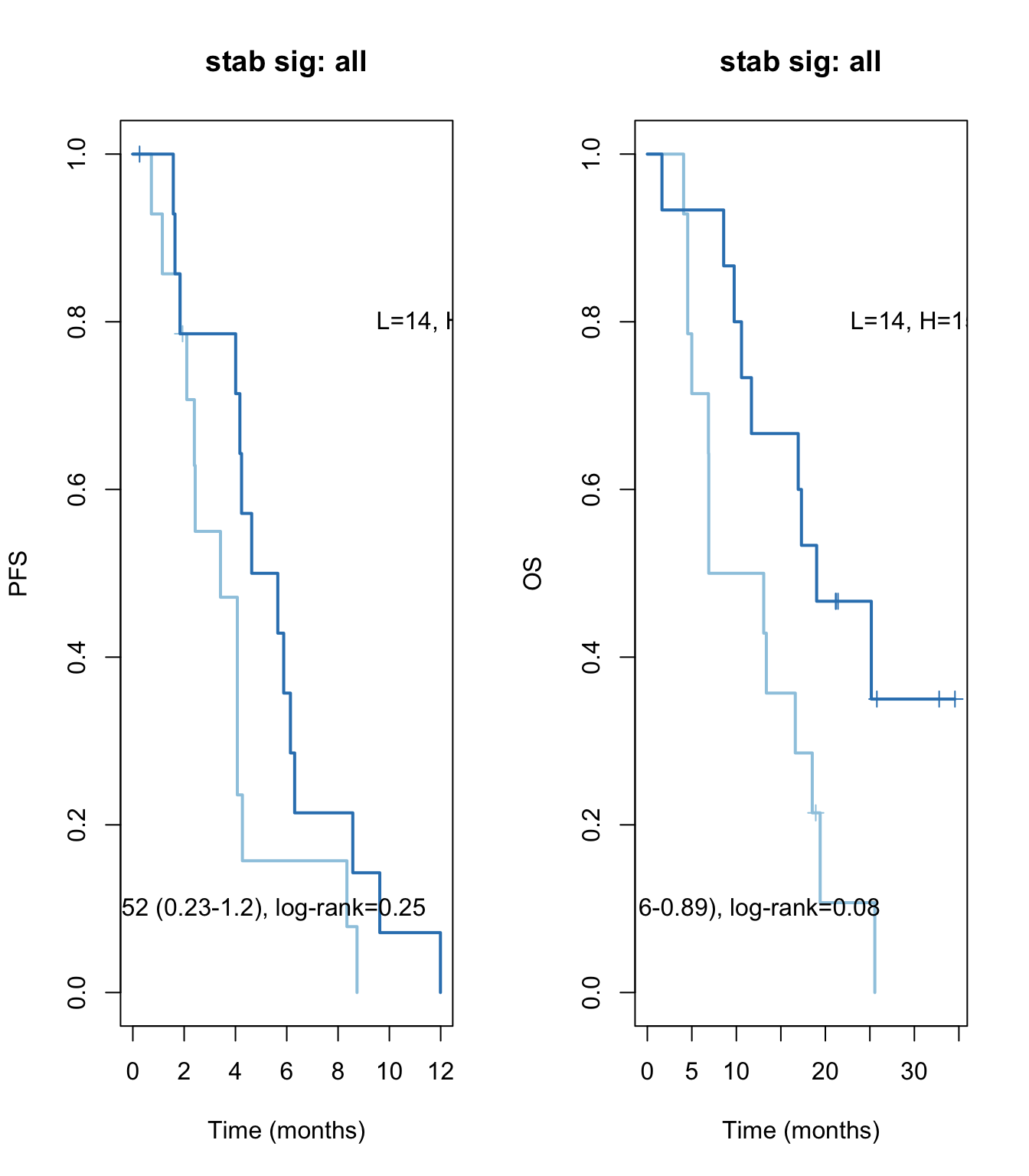
## survival outcome: cts variable
dfs1=coxph(ssPS~stab+Arm, data=newtab)
summary(dfs1)
## Call:
## coxph(formula = ssPS ~ stab + Arm, data = newtab)
##
##   n= 30, number of events= 28
##
##         coef exp(coef) se(coef)      z Pr(>|z|)
## stab -0.2647    0.7675   0.1864 -1.420    0.156
## ArmB  0.4682    1.5971   0.4140  1.131    0.258
##
##      exp(coef) exp(-coef) lower .95 upper .95
## stab    0.7675     1.3030    0.5326     1.106
## ArmB    1.5971     0.6261    0.7095     3.595
##
## Concordance= 0.592  (se = 0.071 )
## Likelihood ratio test= 2.77  on 2 df,   p=0.3
## Wald test            = 2.71  on 2 df,   p=0.3
## Score (logrank) test = 2.78  on 2 df,   p=0.2
os1=coxph(ssOS~stab+Arm, data=newtab)
summary(os1)
## Call:
## coxph(formula = ssOS ~ stab + Arm, data = newtab)
##
##   n= 30, number of events= 22
##
##         coef exp(coef) se(coef)      z Pr(>|z|)
## stab -0.1572    0.8546   0.2208 -0.712    0.477
## ArmB  0.2415    1.2731   0.4558  0.530    0.596
##
##      exp(coef) exp(-coef) lower .95 upper .95
## stab    0.8546     1.1702    0.5544     1.317
## ArmB    1.2731     0.7855    0.5211     3.111
##
## Concordance= 0.557  (se = 0.075 )
## Likelihood ratio test= 0.61  on 2 df,   p=0.7
## Wald test            = 0.6  on 2 df,   p=0.7
## Score (logrank) test = 0.61  on 2 df,   p=0.7
par(mfrow=c(1,2))

TCGAvalCut=cut(newtab$grow, quantile(newtab$grow, c(0, 0.5, 1)), c("L","P"))

dfs1=coxph(ssPS~TCGAvalCut+Arm, data=newtab)
summary(dfs1)
## Call:
## coxph(formula = ssPS ~ TCGAvalCut + Arm, data = newtab)
##
##   n= 29, number of events= 27
##    (1 observation deleted due to missingness)
##
##               coef exp(coef) se(coef)     z Pr(>|z|)
## TCGAvalCutP 0.4793    1.6150   0.4293 1.117    0.264
## ArmB        0.5381    1.7127   0.4380 1.228    0.219
##
##             exp(coef) exp(-coef) lower .95 upper .95
## TCGAvalCutP     1.615     0.6192    0.6963     3.746
## ArmB            1.713     0.5839    0.7258     4.041
##
## Concordance= 0.544  (se = 0.079 )
## Likelihood ratio test= 2.07  on 2 df,   p=0.4
## Wald test            = 2.06  on 2 df,   p=0.4
## Score (logrank) test = 2.06  on 2 df,   p=0.4
adfs=summary(dfs1)
os1=coxph(ssOS~TCGAvalCut+Arm, data=newtab)
summary(os1)
## Call:
## coxph(formula = ssOS ~ TCGAvalCut + Arm, data = newtab)
##
##   n= 29, number of events= 21
##    (1 observation deleted due to missingness)
##
##               coef exp(coef) se(coef)     z Pr(>|z|)
## TCGAvalCutP 0.2460    1.2789   0.5407 0.455    0.649
## ArmB        0.2555    1.2911   0.5356 0.477    0.633
##
##             exp(coef) exp(-coef) lower .95 upper .95
## TCGAvalCutP     1.279     0.7819    0.4432     3.690
## ArmB            1.291     0.7745    0.4519     3.689
##
## Concordance= 0.511  (se = 0.068 )
## Likelihood ratio test= 0.27  on 2 df,   p=0.9
## Wald test            = 0.28  on 2 df,   p=0.9
## Score (logrank) test = 0.28  on 2 df,   p=0.9
aos=summary(os1)

ns=table(TCGAvalCut)
vals=round(c(adfs$conf.int[ 1,c(1, 3:4)], adfs$logtest[3]), 2)
ax2=plot(survfit(ssPS~TCGAvalCut), main=paste("growing sig"), col=brewer.pal(3, "Blues")[2:3],lwd=2, xlab="Time (months)", ylab="PFS", mark.time=T)
text(4, 0.1, sprintf("HR =%s (%s-%s), log-rank=%s",vals[1], vals[2], vals[3], vals[4]))
text(30, 0.8, sprintf("L=%s, H=%s",ns[1], ns[2]))

vals=round(c(aos$conf.int[ 1,c(1, 3:4)], aos$logtest[3]), 2)
ax2=plot(survfit(ssOS~TCGAvalCut), main=paste("growing sig"), col=brewer.pal(3, "Blues")[2:3],lwd=2, xlab="Time (months)", ylab="OS", mark.time=T)
text(4, 0.1, sprintf("HR =%s (%s-%s), log-rank=%s",vals[1], vals[2], vals[3], vals[4]))
text(30, 0.8, sprintf("L=%s, H=%s",ns[1], ns[2]))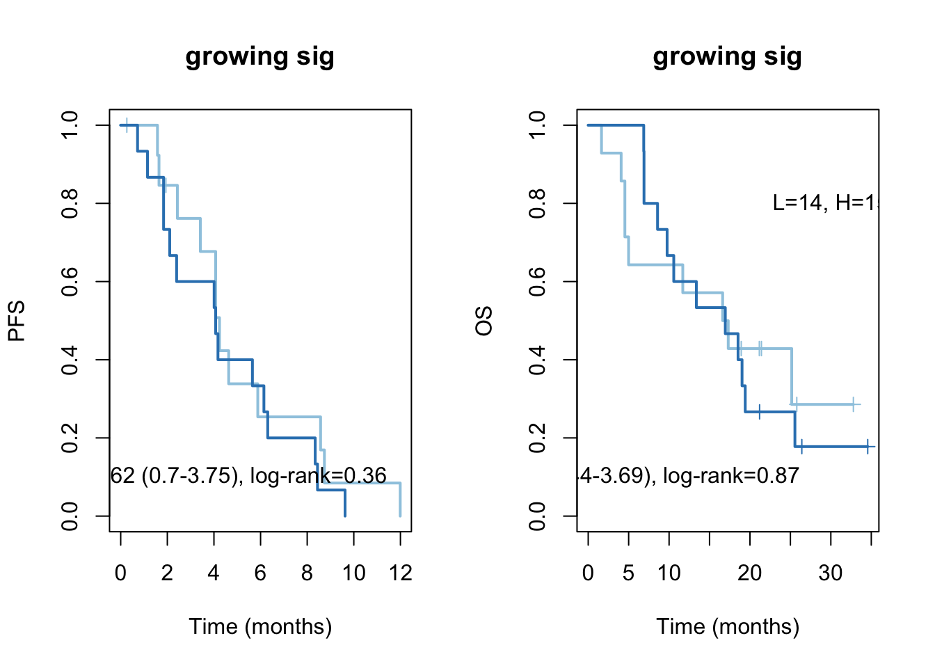
dfs1=coxph(ssPS~grow+Arm, data=newtab)
summary(dfs1)
## Call:
## coxph(formula = ssPS ~ grow + Arm, data = newtab)
##
##   n= 30, number of events= 28
##
##        coef exp(coef) se(coef)     z Pr(>|z|)
## grow 0.1363    1.1461   0.1824 0.747    0.455
## ArmB 0.4490    1.5667   0.4150 1.082    0.279
##
##      exp(coef) exp(-coef) lower .95 upper .95
## grow     1.146     0.8726    0.8015     1.639
## ArmB     1.567     0.6383    0.6946     3.534
##
## Concordance= 0.568  (se = 0.081 )
## Likelihood ratio test= 1.39  on 2 df,   p=0.5
## Wald test            = 1.44  on 2 df,   p=0.5
## Score (logrank) test = 1.45  on 2 df,   p=0.5
os1=coxph(ssOS~grow+Arm, data=newtab)
summary(os1)
## Call:
## coxph(formula = ssOS ~ grow + Arm, data = newtab)
##
##   n= 30, number of events= 22
##
##        coef exp(coef) se(coef)     z Pr(>|z|)
## grow 0.2072    1.2303   0.2565 0.808    0.419
## ArmB 0.3770    1.4578   0.5117 0.737    0.461
##
##      exp(coef) exp(-coef) lower .95 upper .95
## grow     1.230     0.8128    0.7441     2.034
## ArmB     1.458     0.6859    0.5348     3.974
##
## Concordance= 0.511  (se = 0.074 )
## Likelihood ratio test= 0.76  on 2 df,   p=0.7
## Wald test            = 0.78  on 2 df,   p=0.7
## Score (logrank) test = 0.77  on 2 df,   p=0.7
Check what happens when you have treament arm:
TCGAvalCut=cut(newtab$stab, quantile(newtab$stab, c(0, 0.5, 1)), c("L", "P"))

tx=newtab$Arm
par(mfrow=c(1,2))
# ax2=plot(survfit(ssPS~TCGAvalCut+ERClin$Arm[na.omit(ax1)]), main=paste(i, "lum growing"), col=brewer.pal(4, "Blues"),lwd=2, xlab="Time (months)", ylab="PS", mark.time=T)

dfs1=coxph(ssPS[newtab$Arm=="A"]~TCGAvalCut[newtab$Arm=="A"])
summary(dfs1)
## Call:
## coxph(formula = ssPS[newtab$Arm == "A"] ~ TCGAvalCut[newtab$Arm ==
##     "A"])
##
##   n= 13, number of events= 13
##    (1 observation deleted due to missingness)
##
##                                   coef exp(coef) se(coef)      z Pr(>|z|)
## TCGAvalCut[newtab$Arm == "A"]P -0.9221    0.3977   0.6532 -1.412    0.158
##
##                                exp(coef) exp(-coef) lower .95 upper .95
## TCGAvalCut[newtab$Arm == "A"]P    0.3977      2.515    0.1105     1.431
##
## Concordance= 0.597  (se = 0.079 )
## Likelihood ratio test= 1.94  on 1 df,   p=0.2
## Wald test            = 1.99  on 1 df,   p=0.2
## Score (logrank) test = 2.12  on 1 df,   p=0.1
adfs=summary(dfs1)
dfs1=coxph(ssPS[newtab$Arm=="B"]~TCGAvalCut[newtab$Arm=="B"])
summary(dfs1)
## Call:
## coxph(formula = ssPS[newtab$Arm == "B"] ~ TCGAvalCut[newtab$Arm ==
##     "B"])
##
##   n= 16, number of events= 14
##
##                                   coef exp(coef) se(coef)      z Pr(>|z|)
## TCGAvalCut[newtab$Arm == "B"]P -0.5066    0.6026   0.5771 -0.878     0.38
##
##                                exp(coef) exp(-coef) lower .95 upper .95
## TCGAvalCut[newtab$Arm == "B"]P    0.6026       1.66    0.1944     1.867
##
## Concordance= 0.626  (se = 0.08 )
## Likelihood ratio test= 0.77  on 1 df,   p=0.4
## Wald test            = 0.77  on 1 df,   p=0.4
## Score (logrank) test = 0.78  on 1 df,   p=0.4
bdfs=summary(dfs1)

par(mfrow=c(2,2))
## plot separately the different arms
vals=round(c(adfs$conf.int[ 1,c(1, 3:4)], adfs$logtest[3]), 2)
ns=table(TCGAvalCut[newtab$Arm=="A"])
ax2=plot(survfit(ssPS[tx=="A"]~TCGAvalCut[tx=="A"]), main="stable ArmA", col=brewer.pal(3, "Blues")[2:3],lwd=2, xlab="Time (months)", ylab="PS", mark.time=T, xlim=c(0,12))
text(4, 0.1, sprintf("HR =%s (%s-%s), log-rank=%s",vals[1], vals[2], vals[3], vals[4]))
text(10, 0.8, sprintf("L=%s, H=%s",ns[1], ns[2]))
vals=round(c(bdfs$conf.int[ 1,c(1, 3:4)], bdfs$logtest[3]), 2)
ns=table(TCGAvalCut[newtab$Arm=="B"])
ax2=plot(survfit(ssPS[tx=="B"]~TCGAvalCut[tx=="B"]), main="stable ArmB", col=brewer.pal(3, "Blues")[2:3],lwd=2, xlab="Time (months)", ylab="PS", mark.time=T, xlim=c(0, 12))
text(4, 0.1, sprintf("HR =%s (%s-%s), log-rank=%s",vals[1], vals[2], vals[3], vals[4]))
text(10, 0.8, sprintf("L=%s, H=%s",ns[1], ns[2]))

## plot the OS result
# OS based on arm: stable

dfs1=coxph(ssOS[newtab$Arm=="A"]~TCGAvalCut[newtab$Arm=="A"])
summary(dfs1)
## Call:
## coxph(formula = ssOS[newtab$Arm == "A"] ~ TCGAvalCut[newtab$Arm ==
##     "A"])
##
##   n= 13, number of events= 10
##    (1 observation deleted due to missingness)
##
##                                   coef exp(coef) se(coef)      z Pr(>|z|)
## TCGAvalCut[newtab$Arm == "A"]P -0.5760    0.5622   0.6418 -0.897     0.37
##
##                                exp(coef) exp(-coef) lower .95 upper .95
## TCGAvalCut[newtab$Arm == "A"]P    0.5622      1.779    0.1598     1.978
##
## Concordance= 0.555  (se = 0.088 )
## Likelihood ratio test= 0.8  on 1 df,   p=0.4
## Wald test            = 0.81  on 1 df,   p=0.4
## Score (logrank) test = 0.83  on 1 df,   p=0.4
adfs=summary(dfs1)
dfs1=coxph(ssOS[newtab$Arm=="B"]~TCGAvalCut[newtab$Arm=="B"])
summary(dfs1)
## Call:
## coxph(formula = ssOS[newtab$Arm == "B"] ~ TCGAvalCut[newtab$Arm ==
##     "B"])
##
##   n= 16, number of events= 12
##
##                                   coef exp(coef) se(coef)      z Pr(>|z|)
## TCGAvalCut[newtab$Arm == "B"]P -1.5044    0.2222   0.6941 -2.167   0.0302 *
## ---
## Signif. codes:  0 '***' 0.001 '**' 0.01 '*' 0.05 '.' 0.1 ' ' 1
##
##                                exp(coef) exp(-coef) lower .95 upper .95
## TCGAvalCut[newtab$Arm == "B"]P    0.2222      4.501     0.057    0.8659
##
## Concordance= 0.694  (se = 0.054 )
## Likelihood ratio test= 5.39  on 1 df,   p=0.02
## Wald test            = 4.7  on 1 df,   p=0.03
## Score (logrank) test = 5.5  on 1 df,   p=0.02
bdfs=summary(dfs1)

## plot separately the different arms
vals=round(c(adfs$conf.int[ 1,c(1, 3:4)], adfs$logtest[3]), 2)
ns=table(TCGAvalCut[newtab$Arm=="A"])
ax2=plot(survfit(ssOS[tx=="A"]~TCGAvalCut[tx=="A"]), main="stable ArmA", col=brewer.pal(3, "Blues")[2:3],lwd=2, xlab="Time (months)", ylab="OS", mark.time=T, xlim=c(0, 35))
text(4, 0.1, sprintf("HR =%s (%s-%s), log-rank=%s",vals[1], vals[2], vals[3], vals[4]))
text(30, 0.8, sprintf("L=%s, H=%s",ns[1], ns[2]))

vals=round(c(bdfs$conf.int[ 1,c(1, 3:4)], bdfs$logtest[3]), 2)
ns=table(TCGAvalCut[newtab$Arm=="B"])
ax2=plot(survfit(ssOS[tx=="B"]~TCGAvalCut[tx=="B"]), main="stable ArmB", col=brewer.pal(3, "Blues")[2:3],lwd=2, xlab="Time (months)", ylab="OS", mark.time=T, xlim=c(0, 35))
text(4, 0.1, sprintf("HR =%s (%s-%s), log-rank=%s",vals[1], vals[2], vals[3], vals[4]))
text(30, 0.8, sprintf("L=%s, H=%s",ns[1], ns[2]))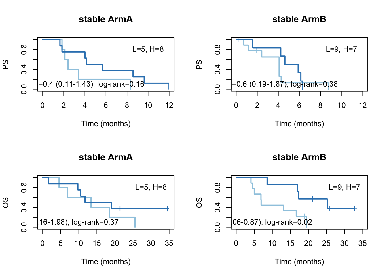
TCGAvalCut=cut(newtab$grow, c(-10, median(newtab$grow), 10), c("L", "P"))

# ax2=plot(survfit(ssPS~TCGAvalCut+ERClin$Arm[na.omit(ax1)]), main=paste(i, "lum growing"), col=brewer.pal(4, "Blues"),lwd=2, xlab="Time (months)", ylab="PS", mark.time=T)

dfs1=coxph(ssPS[newtab$Arm=="A"]~TCGAvalCut[newtab$Arm=="A"])
summary(dfs1)
## Call:
## coxph(formula = ssPS[newtab$Arm == "A"] ~ TCGAvalCut[newtab$Arm ==
##     "A"])
##
##   n= 14, number of events= 14
##
##                                  coef exp(coef) se(coef)     z Pr(>|z|)
## TCGAvalCut[newtab$Arm == "A"]P 0.6467    1.9092   0.6795 0.952    0.341
##
##                                exp(coef) exp(-coef) lower .95 upper .95
## TCGAvalCut[newtab$Arm == "A"]P     1.909     0.5238     0.504     7.232
##
## Concordance= 0.533  (se = 0.093 )
## Likelihood ratio test= 1  on 1 df,   p=0.3
## Wald test            = 0.91  on 1 df,   p=0.3
## Score (logrank) test = 0.93  on 1 df,   p=0.3
adfs=summary(dfs1)
dfs1=coxph(ssPS[newtab$Arm=="B"]~TCGAvalCut[newtab$Arm=="B"])
summary(dfs1)
## Call:
## coxph(formula = ssPS[newtab$Arm == "B"] ~ TCGAvalCut[newtab$Arm ==
##     "B"])
##
##   n= 16, number of events= 14
##
##                                  coef exp(coef) se(coef)     z Pr(>|z|)
## TCGAvalCut[newtab$Arm == "B"]P 0.1065    1.1123   0.5883 0.181    0.856
##
##                                exp(coef) exp(-coef) lower .95 upper .95
## TCGAvalCut[newtab$Arm == "B"]P     1.112      0.899    0.3511     3.524
##
## Concordance= 0.549  (se = 0.098 )
## Likelihood ratio test= 0.03  on 1 df,   p=0.9
## Wald test            = 0.03  on 1 df,   p=0.9
## Score (logrank) test = 0.03  on 1 df,   p=0.9
bdfs=summary(dfs1)

par(mfrow=c(2,2))
## plot separately the different arms
ns=table(TCGAvalCut[newtab$Arm=="A"])
vals=round(c(adfs$conf.int[ 1,c(1, 3:4)], adfs$logtest[3]), 2)
ax2=plot(survfit(ssPS[tx=="A"]~TCGAvalCut[tx=="A"]), main="grow ArmA", col=brewer.pal(3, "Blues")[2:3],lwd=2, xlab="Time (months)", ylab="PS", mark.time=T)
text(4, 0.1, sprintf("HR =%s (%s-%s), log-rank=%s",vals[1], vals[2], vals[3], vals[4]))
text(12, 0.8, sprintf("L=%s, H=%s",ns[1], ns[2]))
ns=table(TCGAvalCut[newtab$Arm=="B"])
vals=round(c(bdfs$conf.int[ 1,c(1, 3:4)], bdfs$logtest[3]), 2)
ax2=plot(survfit(ssPS[tx=="B"]~TCGAvalCut[tx=="B"]), main="grow ArmB", col=brewer.pal(3, "Blues")[2:3],lwd=2, xlab="Time (months)", ylab="PS", mark.time=T)
text(4, 0.1, sprintf("HR =%s (%s-%s), log-rank=%s",vals[1], vals[2], vals[3], vals[4]))
text(12, 0.8, sprintf("L=%s, H=%s",ns[1], ns[2]))


## plot the OS result
# OS based on arm: stable

dfs1=coxph(ssOS[newtab$Arm=="A"]~TCGAvalCut[newtab$Arm=="A"])
summary(dfs1)
## Call:
## coxph(formula = ssOS[newtab$Arm == "A"] ~ TCGAvalCut[newtab$Arm ==
##     "A"])
##
##   n= 14, number of events= 10
##
##                                   coef exp(coef) se(coef)      z Pr(>|z|)
## TCGAvalCut[newtab$Arm == "A"]P -0.7614    0.4670   0.7141 -1.066    0.286
##
##                                exp(coef) exp(-coef) lower .95 upper .95
## TCGAvalCut[newtab$Arm == "A"]P     0.467      2.141    0.1152     1.893
##
## Concordance= 0.608  (se = 0.084 )
## Likelihood ratio test= 1.03  on 1 df,   p=0.3
## Wald test            = 1.14  on 1 df,   p=0.3
## Score (logrank) test = 1.19  on 1 df,   p=0.3
adfs=summary(dfs1)
dfs1=coxph(ssOS[newtab$Arm=="B"]~TCGAvalCut[newtab$Arm=="B"])
summary(dfs1)
## Call:
## coxph(formula = ssOS[newtab$Arm == "B"] ~ TCGAvalCut[newtab$Arm ==
##     "B"])
##
##   n= 16, number of events= 12
##
##                                  coef exp(coef) se(coef)     z Pr(>|z|)
## TCGAvalCut[newtab$Arm == "B"]P 0.8206    2.2718   0.6166 1.331    0.183
##
##                                exp(coef) exp(-coef) lower .95 upper .95
## TCGAvalCut[newtab$Arm == "B"]P     2.272     0.4402    0.6785     7.607
##
## Concordance= 0.563  (se = 0.071 )
## Likelihood ratio test= 1.69  on 1 df,   p=0.2
## Wald test            = 1.77  on 1 df,   p=0.2
## Score (logrank) test = 1.86  on 1 df,   p=0.2
bdfs=summary(dfs1)

## plot separately the different arms
vals=round(c(adfs$conf.int[ 1,c(1, 3:4)], adfs$logtest[3]), 2)
ns=table(TCGAvalCut[newtab$Arm=="A"])
ax2=plot(survfit(ssOS[tx=="A"]~TCGAvalCut[tx=="A"]), main="grow ArmA", col=brewer.pal(3, "Blues")[2:3],lwd=2, xlab="Time (months)", ylab="OS", mark.time=T)
text(4, 0.1, sprintf("HR =%s (%s-%s), log-rank=%s",vals[1], vals[2], vals[3], vals[4]))
text(30, 0.8, sprintf("L=%s, H=%s",ns[1], ns[2]))
ns=table(TCGAvalCut[newtab$Arm=="B"])
vals=round(c(bdfs$conf.int[ 1,c(1, 3:4)], bdfs$logtest[3]), 2)
ax2=plot(survfit(ssOS[tx=="B"]~TCGAvalCut[tx=="B"]), main="grow ArmB", col=brewer.pal(3, "Blues")[2:3],lwd=2, xlab="Time (months)", ylab="OS", mark.time=T)
text(4, 0.1, sprintf("HR =%s (%s-%s), log-rank=%s",vals[1], vals[2], vals[3], vals[4]))
text(30, 0.8, sprintf("L=%s, H=%s",ns[1], ns[2]))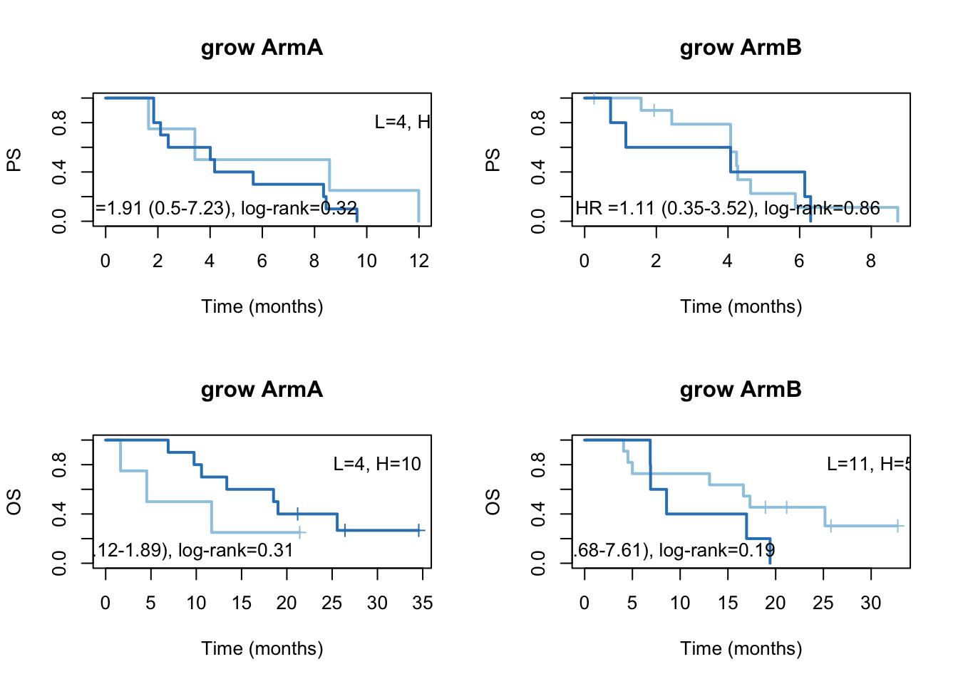
Note that the ams are imbalanced, do this again after splitting accord to median in both groups
tx=which(newtab$Arm=="A")
TCGAvalCut=cut(newtab$grow[tx], c(-10, median(newtab$grow[tx]), 10), c("L", "P"))

# ax2=plot(survfit(ssPS~TCGAvalCut+ERClin$Arm[na.omit(ax1)]), main=paste(i, "lum growing"), col=brewer.pal(4, "Blues"),lwd=2, xlab="Time (months)", ylab="PS", mark.time=T)

dfs1=coxph(ssPS[tx]~TCGAvalCut)
summary(dfs1)
adfs=summary(dfs1)

dfs1=coxph(ssOS[tx]~TCGAvalCut)
summary(dfs1)
aos=summary(dfs1)

par(mfrow=c(2,2))
## plot separately the different arms
vals=round(c(adfs$conf.int[ 1,c(1, 3:4)], adfs$logtest[3]), 2)
ns=table(TCGAvalCut)

ax2=plot(survfit(ssPS[tx]~TCGAvalCut), main="grow ArmA", col=brewer.pal(3, "Blues")[2:3],lwd=2, xlab="Time (months)", ylab="PS", mark.time=T)
text(4, 0.1, sprintf("HR =%s (%s-%s), log-rank=%s",vals[1], vals[2], vals[3], vals[4]))
text(12, 0.8, sprintf("L=%s, H=%s",ns[1], ns[2]))

vals=round(c(aos$conf.int[ 1,c(1, 3:4)], aos$logtest[3]), 2)
ax2=plot(survfit(ssOS[tx]~TCGAvalCut), main="grow ArmA", col=brewer.pal(3, "Blues")[2:3],lwd=2, xlab="Time (months)", ylab="OS", mark.time=T)
text(15, 0.1, sprintf("HR =%s (%s-%s), log-rank=%s",vals[1], vals[2], vals[3], vals[4]))
text(30, 0.8, sprintf("L=%s, H=%s",ns[1], ns[2]))

## plot the OS result
# OS based on arm: stable

tx=which(newtab$Arm=="B")
TCGAvalCut=cut(newtab$grow[tx], c(-10, median(newtab$grow[tx]), 10), c("L", "P"))


dfs1=coxph(ssOS[newtab$Arm=="B"]~TCGAvalCut)
summary(dfs1)
bos=summary(dfs1)
dfs1=coxph(ssPS[newtab$Arm=="B"]~TCGAvalCut)
summary(dfs1)
bdfs=summary(dfs1)
ns=table(TCGAvalCut)
## plot separately the different arms
vals=round(c(bdfs$conf.int[ 1,c(1, 3:4)], bdfs$logtest[3]), 2)
ax2=plot(survfit(ssPS[tx]~TCGAvalCut), main="grow ArmB", col=brewer.pal(3, "Blues")[2:3],lwd=2, xlab="Time (months)", ylab="PS", mark.time=T, xlim=c(0, 12))
text(4, 0.1, sprintf("HR =%s (%s-%s), log-rank=%s",vals[1], vals[2], vals[3], vals[4]))
text(12, 0.8, sprintf("L=%s, H=%s",ns[1], ns[2]))

vals=round(c(bos$conf.int[ 1,c(1, 3:4)], bos$logtest[3]), 2)
ax2=plot(survfit(ssOS[tx]~TCGAvalCut), main="grow ArmB", col=brewer.pal(3, "Blues")[2:3],lwd=2, xlab="Time (months)", ylab="OS", mark.time=T, xlim=c(0, 35))
text(15, 0.1, sprintf("HR =%s (%s-%s), log-rank=%s",vals[1], vals[2], vals[3], vals[4]))
text(30, 0.8, sprintf("L=%s, H=%s",ns[1], ns[2]))
tx=which(newtab$Arm=="A")
TCGAvalCut=cut(newtab$stab[tx], c(-10, median(newtab$stab[tx]), 10), c("L", "P"))

# ax2=plot(survfit(ssPS~TCGAvalCut+ERClin$Arm[na.omit(ax1)]), main=paste(i, "lum growing"), col=brewer.pal(4, "Blues"),lwd=2, xlab="Time (months)", ylab="PS", mark.time=T)

dfs1=coxph(ssPS[tx]~TCGAvalCut)
summary(dfs1)
adfs=summary(dfs1)

dfs1=coxph(ssOS[tx]~TCGAvalCut)
summary(dfs1)
aos=summary(dfs1)

par(mfrow=c(2,2))
## plot separately the different arms
vals=round(c(adfs$conf.int[ 1,c(1, 3:4)], adfs$logtest[3]), 2)
ns=table(TCGAvalCut)

ax2=plot(survfit(ssPS[tx]~TCGAvalCut), main="stab ArmA", col=brewer.pal(3, "Blues")[2:3],lwd=2, xlab="Time (months)", ylab="PS", mark.time=T)
text(4, 0.1, sprintf("HR =%s (%s-%s), log-rank=%s",vals[1], vals[2], vals[3], vals[4]))
text(12, 0.8, sprintf("L=%s, H=%s",ns[1], ns[2]))

vals=round(c(aos$conf.int[ 1,c(1, 3:4)], aos$logtest[3]), 2)
ax2=plot(survfit(ssOS[tx]~TCGAvalCut), main="stab ArmA", col=brewer.pal(3, "Blues")[2:3],lwd=2, xlab="Time (months)", ylab="OS", mark.time=T)
text(15, 0.1, sprintf("HR =%s (%s-%s), log-rank=%s",vals[1], vals[2], vals[3], vals[4]))
text(30, 0.8, sprintf("L=%s, H=%s",ns[1], ns[2]))

## plot the OS result
# OS based on arm: stable

tx=which(newtab$Arm=="B")
TCGAvalCut=cut(newtab$stab[tx], c(-10, median(newtab$stab[tx]), 10), c("L", "P"))


dfs1=coxph(ssOS[newtab$Arm=="B"]~TCGAvalCut)
summary(dfs1)
bos=summary(dfs1)
dfs1=coxph(ssPS[newtab$Arm=="B"]~TCGAvalCut)
summary(dfs1)
bdfs=summary(dfs1)
ns=table(TCGAvalCut)
## plot separately the different arms
vals=round(c(bdfs$conf.int[ 1,c(1, 3:4)], bdfs$logtest[3]), 2)
ax2=plot(survfit(ssPS[tx]~TCGAvalCut), main="stab ArmB", col=brewer.pal(3, "Blues")[2:3],lwd=2, xlab="Time (months)", ylab="PS", mark.time=T, xlim=c(0, 12))
text(4, 0.1, sprintf("HR =%s (%s-%s), log-rank=%s",vals[1], vals[2], vals[3], vals[4]))
text(12, 0.8, sprintf("L=%s, H=%s",ns[1], ns[2]))

vals=round(c(bos$conf.int[ 1,c(1, 3:4)], bos$logtest[3]), 2)
ax2=plot(survfit(ssOS[tx]~TCGAvalCut), main="stab ArmB", col=brewer.pal(3, "Blues")[2:3],lwd=2, xlab="Time (months)", ylab="OS", mark.time=T, xlim=c(0, 35))
text(15, 0.1, sprintf("HR =%s (%s-%s), log-rank=%s",vals[1], vals[2], vals[3], vals[4]))
text(30, 0.8, sprintf("L=%s, H=%s",ns[1], ns[2]))
16.2 Do associative study with other features?
# growing signature
TCGAvalCut=cut(newtab$grow, c(-10, median(newtab$grow), 10), c("L", "H"))

table(TCGAvalCut, newtab$PDL1)
##
## TCGAvalCut    Negative Positive
##          L  1        6        8
##          H  0       11        4
m1=matrix(c(6, 8, 11, 4), ncol=2)
chisq.test(m1)
##
##  Pearson's Chi-squared test with Yates' continuity correction
##
## data:  m1
## X-squared = 1.6587, df = 1, p-value = 0.1978

table(TCGAvalCut, newtab$Arm)
##
## TCGAvalCut  A  B
##          L  4 11
##          H 10  5
chisq.test(table(TCGAvalCut, newtab$Arm))
##
##  Pearson's Chi-squared test with Yates' continuity correction
##
## data:  table(TCGAvalCut, newtab$Arm)
## X-squared = 3.3482, df = 1, p-value = 0.06728

table(TCGAvalCut,newtab$ClinBen)
##
## TCGAvalCut  0  1
##          L 10  5
##          H  9  6
chisq.test(table(TCGAvalCut,newtab$ClinBen))
##
##  Pearson's Chi-squared test with Yates' continuity correction
##
## data:  table(TCGAvalCut, newtab$ClinBen)
## X-squared = 0, df = 1, p-value = 1

table(TCGAvalCut,newtab$Response)
##
## TCGAvalCut NE PD PR SD
##          L  2  3  4  6
##          H  1  5  4  5

chisq.test(table(TCGAvalCut,newtab$Response))
##
##  Pearson's Chi-squared test
##
## data:  table(TCGAvalCut, newtab$Response)
## X-squared = 0.92424, df = 3, p-value = 0.8196
boxplot the growing scores with other covariates:
par(mfrow=c(2,3))
plot(newtab$grow, newtab$Purity, ylab="Purity", xlab="signature")
plot(newtab$grow, newtab$CD8, ylab="CIBERSORT CD8", xlab="signature")
plot(newtab$grow, newtab$DC, ylab="CIBERSORT DC", xlab="signature")
plot(newtab$grow,newtab$TMB, ylab="TMB", xlab="signature")
boxplot(newtab$grow[newtab$Arm=="A"] ~ newtab$Response[newtab$Arm=="A"], main="Arm A", ylab="signature")
boxplot(newtab$grow[newtab$Arm=="B"] ~ newtab$Response[newtab$Arm=="B"], main="Arm B", ylab="signature")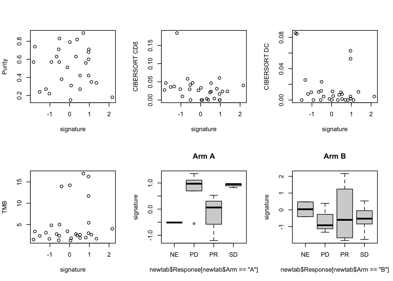
#plot(newtab$grow, newtab$MICB)
#plot(newtab$grow, newtab$MICA, xlab="Signature", ylab="MICA", pch=19)
boxplot(newtab$TMB~TCGAvalCut)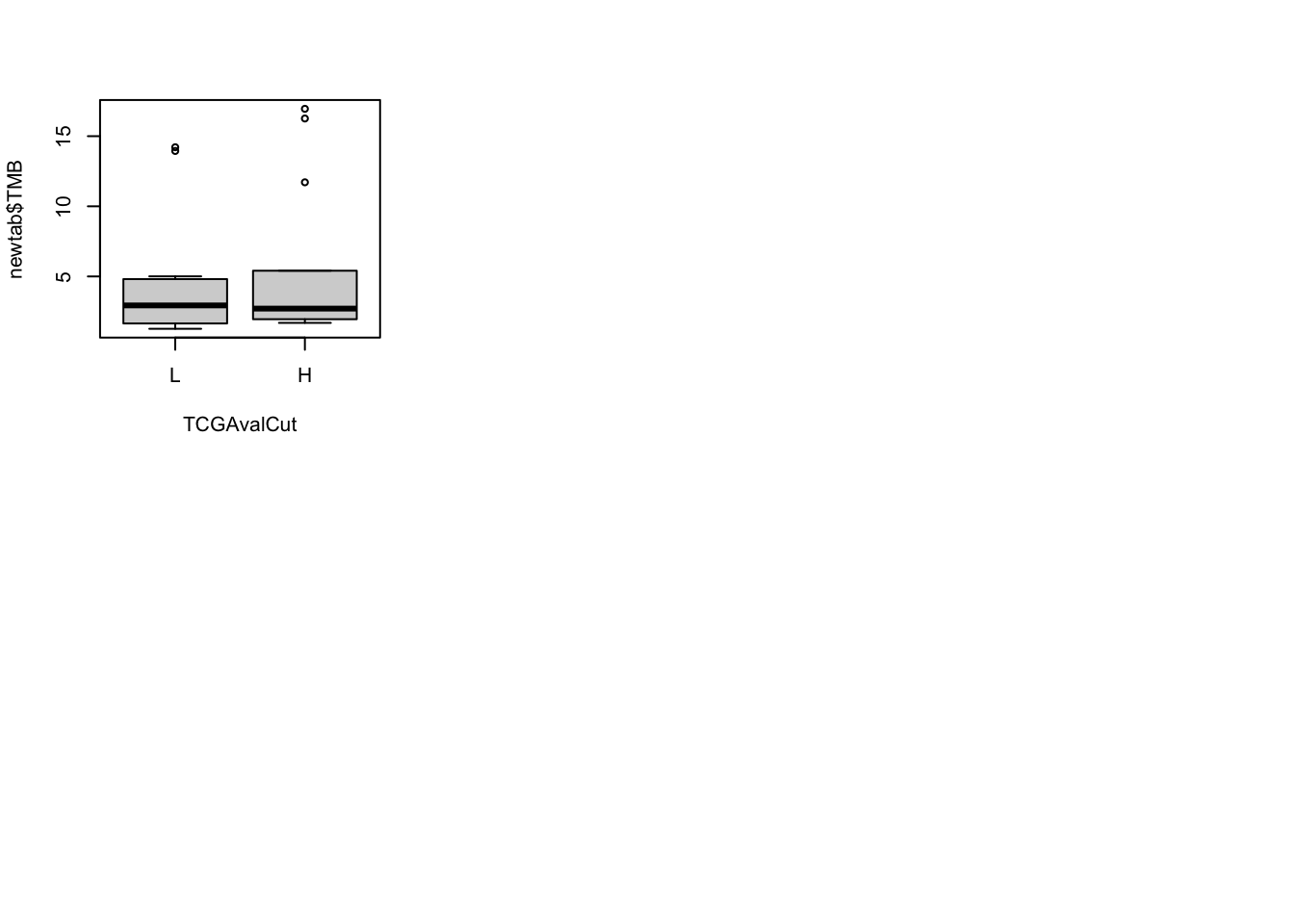
Check the association between expression of the growing signatrue and the cytokines profiled
ERcyt2=ERcytokines[which(ERcytokines$Time=="Pre"), ]
ERcyt2$grow=newtab$grow[match(paste("Patient", ERcyt2$Subject.ID, sep=""), rownames(newtab))]
ERcyt3=ERcytokines[which(ERcytokines$Time=="Post"), ]
ERcyt2$MICA_post=ERcyt3$MICA[match(ERcyt2$Subject.ID, ERcyt3$Subject.ID)]
ERcyt2$MICB_post=ERcyt3$MICB[match(ERcyt2$Subject.ID, ERcyt3$Subject.ID)]

CorVals=sapply(c(6:19, 21:22), function(x) cor(ERcyt2[ ,x], ERcyt2$grow, use="complete", method="spearman" ))
PVals=sapply(c(6:19, 21:22), function(x) cor.test(ERcyt2[ ,x], ERcyt2$grow, use="complete",method="spearman" )$p.value)

names(CorVals)=colnames(ERcyt2)[c(6:19, 21:22)]
names(PVals)=colnames(ERcyt2)[c(6:19, 21:22)]

par(mfrow=c(2,2))
plot(ERcyt2$grow, ERcyt2$MICA, xlab="Signature", ylab="MICA pre", pch=19, ylim=c(0,300))
text(1,250, sprintf("cor=%s, p=%s", round(CorVals[9],2), round(PVals[9],3) ))
plot(ERcyt2$grow, (ERcyt2$MICA_post), xlab="Signature", ylab="MICA post", pch=19, ylim=c(0, 300))
text(1,250, sprintf("cor=%s, p=%s", round(CorVals[15],2), round(PVals[15],3) ))
plot(ERcyt2$grow, ERcyt2$MICB, xlab="Signature", ylab="MICB pre", pch=19, ylim=c(0, 300))
text(1,250, sprintf("cor=%s, p=%s", round(CorVals[10],2), round(PVals[10],3) ))
plot(ERcyt2$grow, (ERcyt2$MICB_post), xlab="Signature", ylab="MICB post", pch=19, ylim=c(0, 300))
text(1,250, sprintf("cor=%s, p=%s", round(CorVals[16],2), round(PVals[16],3) ))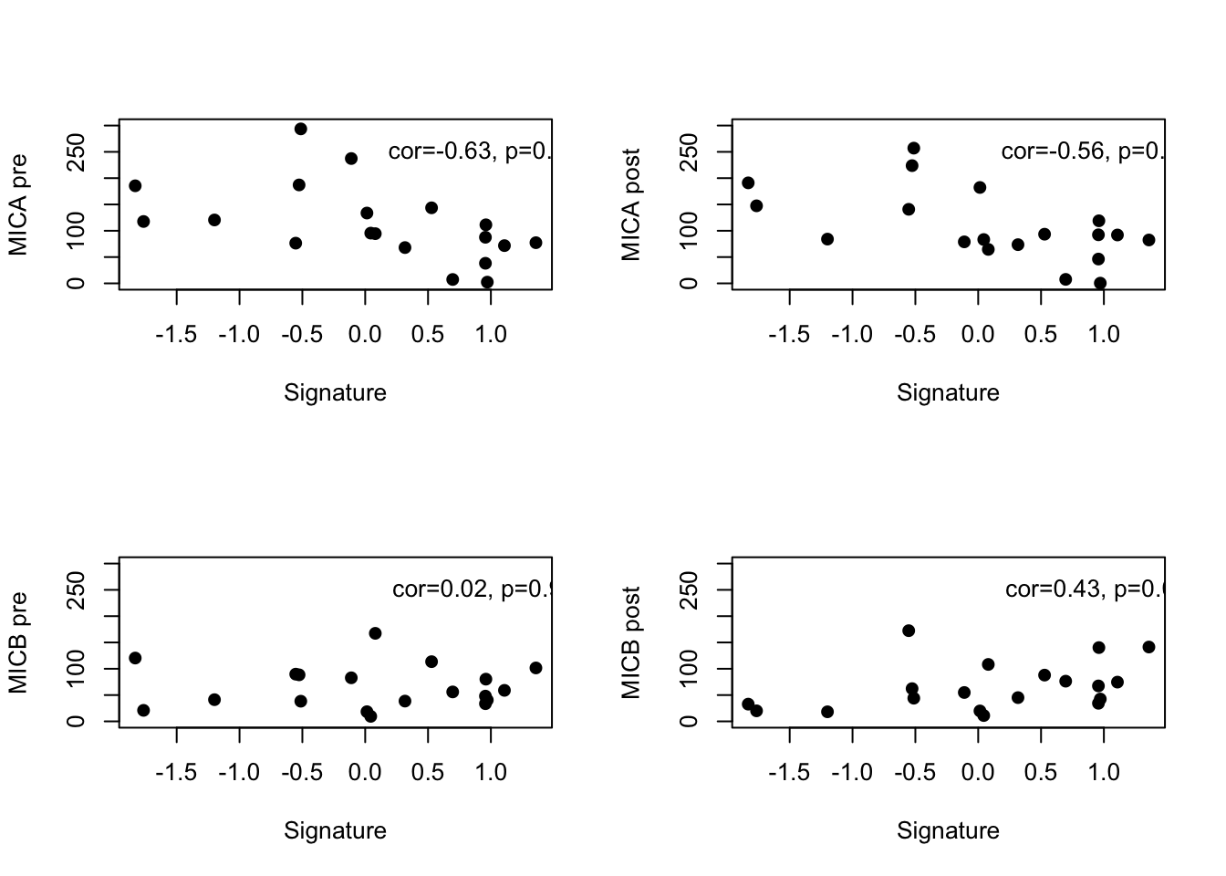
#text(1,250, sprintf("cor=%s, p=%s", round(CorVals[9],2), round(PVals[9],3) ))

par(mfrow=c(1,2))
plot(ERcyt2$grow, (ERcyt2$MICB+ERcyt2$MICA), xlab="Signature", ylab="MICA+MICB_pre", pch=19,
     ylim=c(0, 400))
plot(ERcyt2$grow, (ERcyt2$MICB_post+ERcyt2$MICA_post), xlab="Signature", ylab="MICA+MICB_post", pch=19,
     ylim=c(0, 400))
text(1,250, sprintf("cor=%s, p=%s", round(CorVals[10],2), round(PVals[10],3) ))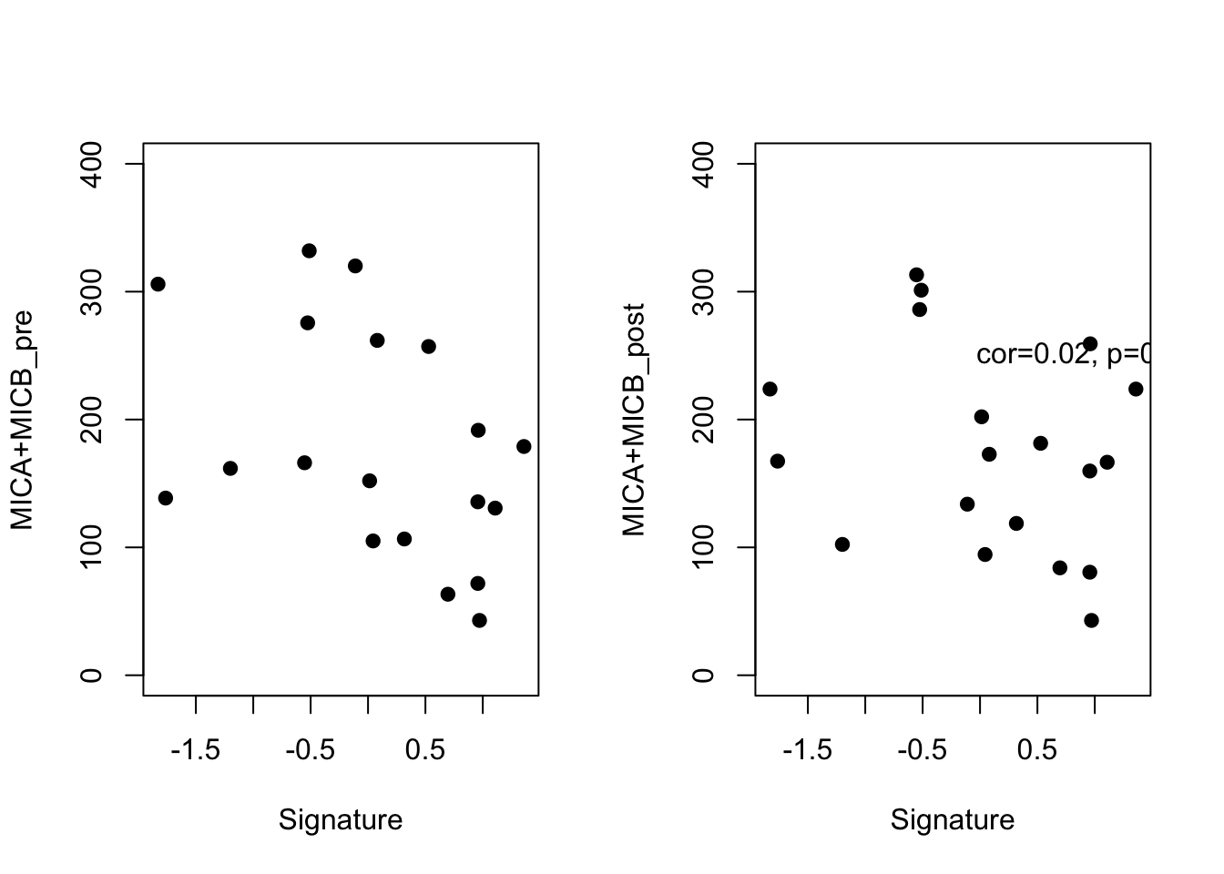
16.3 Use raw counts and perform a batch correction if necessary
Note there are 4 samples whose profiles are out of the ordinary:
ax1=match(colnames(ERcounts)[-1], paste("Patient", ERClin$Subject.ID, sep=""))

colDat=ERClin[ax1, ]
colDat$Sample=paste("Patient", colDat$Subject.ID, sep="")
ddER=DESeqDataSetFromMatrix(countData=round(ERcounts[ ,-1]), colDat=colDat, design=~Arm)
ddER=DESeq(ddER)

ddERvst=vst(ddER)
plotPCA(ddERvst,"Arm")+geom_label(aes(label = name))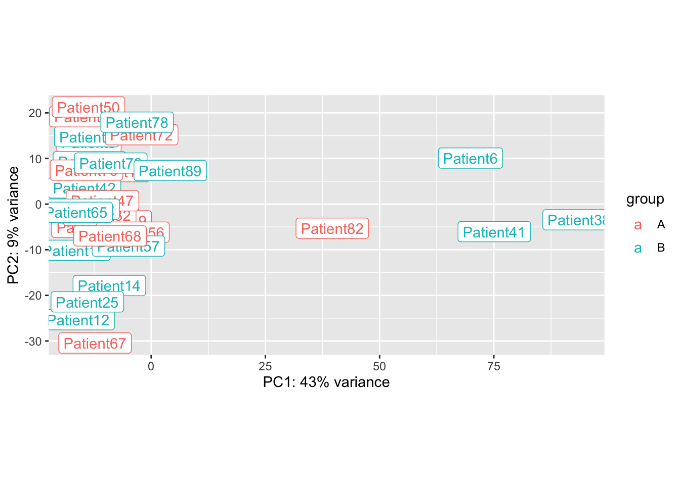
## Do a batch correction based on these 4 patients:

ddERvst$Batch=1
ddERvst$Batch[which(ddERvst$Subject.ID%in%c(6, 82, 41, 38))]=2
#ddERvst$Batch=factor(ddERvst$Batch)

assay(ddERvst)=limma::removeBatchEffect(assay(ddERvst),ddERvst$Batch)

plotPCA(ddERvst,"Arm")+geom_label(aes(label = name))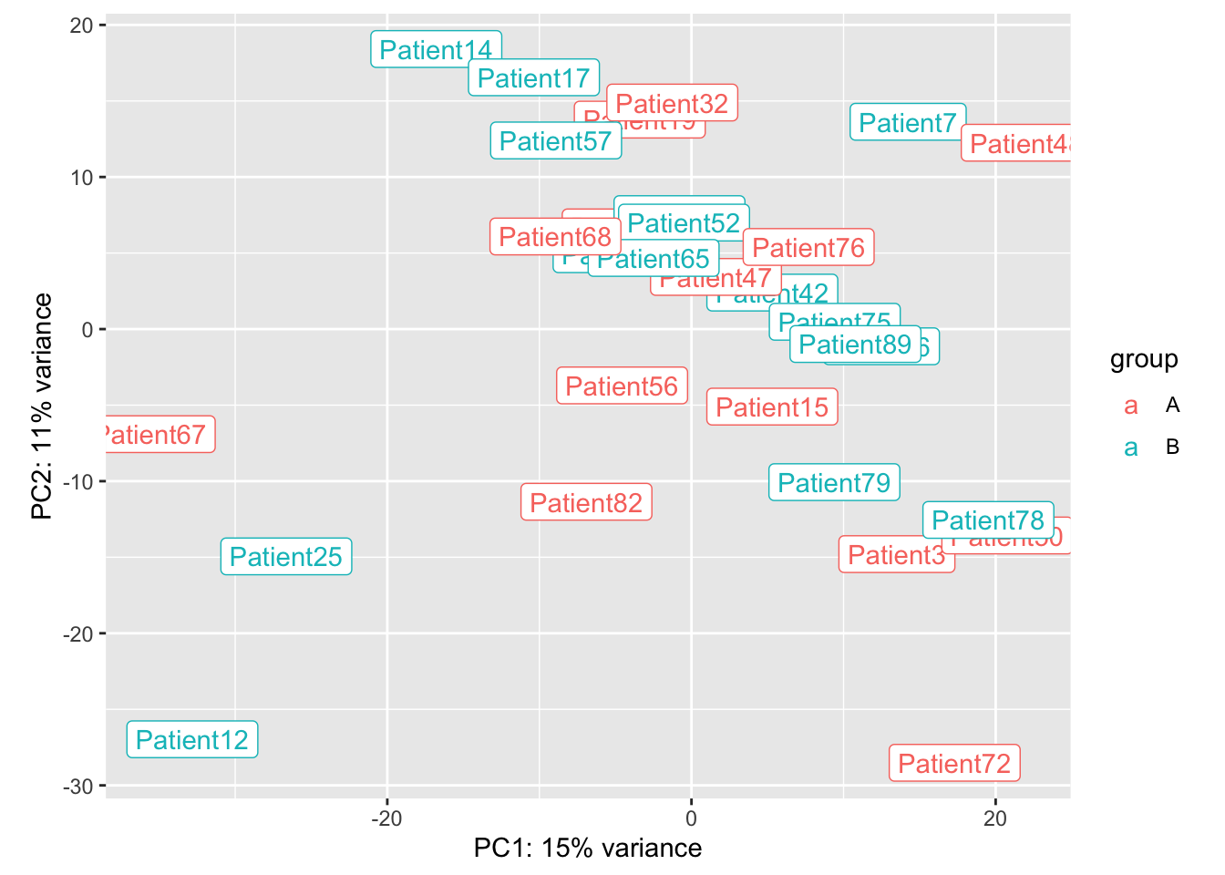
After correction, can we use these values in a ssGSEA
ERssgsea=GSVA::gsva(assay(ddERvst), list(grow=na.omit(HumGeneList2),
stab=Rat2Hum$HGNC.symbol[match(Glistnon, Rat2Hum$RGD.symbol)],Onco=Oncoprint[[1]], Mamma=Oncoprint[[2]]), method="ssgsea", ssgsea.norm=F)ax1=match(colnames(ERssgsea), paste("Patient", ERClin$Subject.ID, sep=""))
ax3=which(!is.na(ax1))
ssPS=Surv(ERClin$PFS.Months[na.omit(ax1)], ERClin$Progression[na.omit(ax1)])
ssOS=Surv(ERClin$OS.Months[na.omit(ax1)], ERClin$Death[na.omit(ax1)] )
ArmInfo=ERClin$Arm[na.omit(ax1)]
PDL1info=ERClin$PD.L1[na.omit(ax1)]
Purity=ERClin$Purity[na.omit(ax1)]
plot(ERssgsea[2, ax3]~Purity)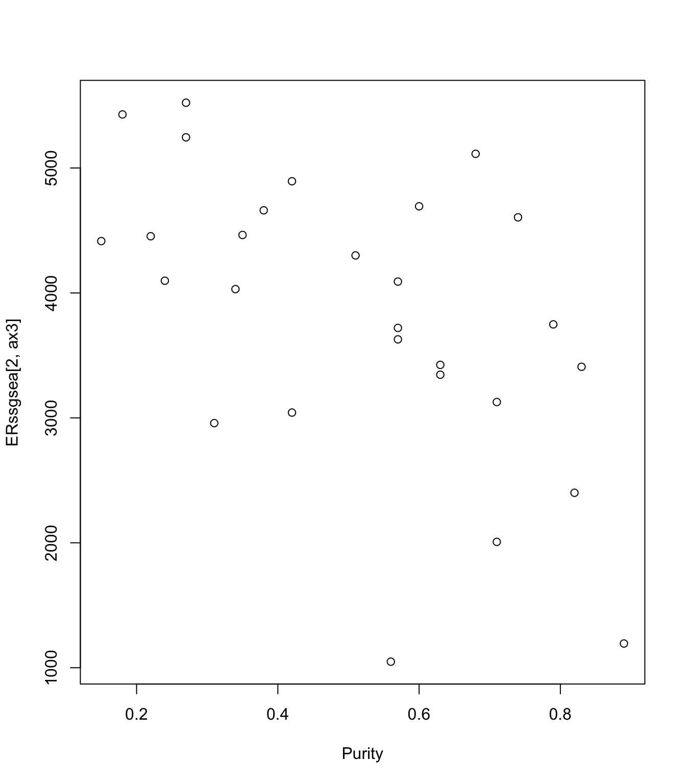
TCGAvalCut=cut(ERssgsea[1,ax3 ], quantile(ERssgsea[1,ax3], c(0, 0.33,0.67, 1)), c("L","M", "P"))

ax2=plot(survfit(ssPS~TCGAvalCut), main=paste(i, "lum growing"), col=brewer.pal(3, "Blues"),lwd=2, xlab="Time (months)", ylab="PS", mark.time=T)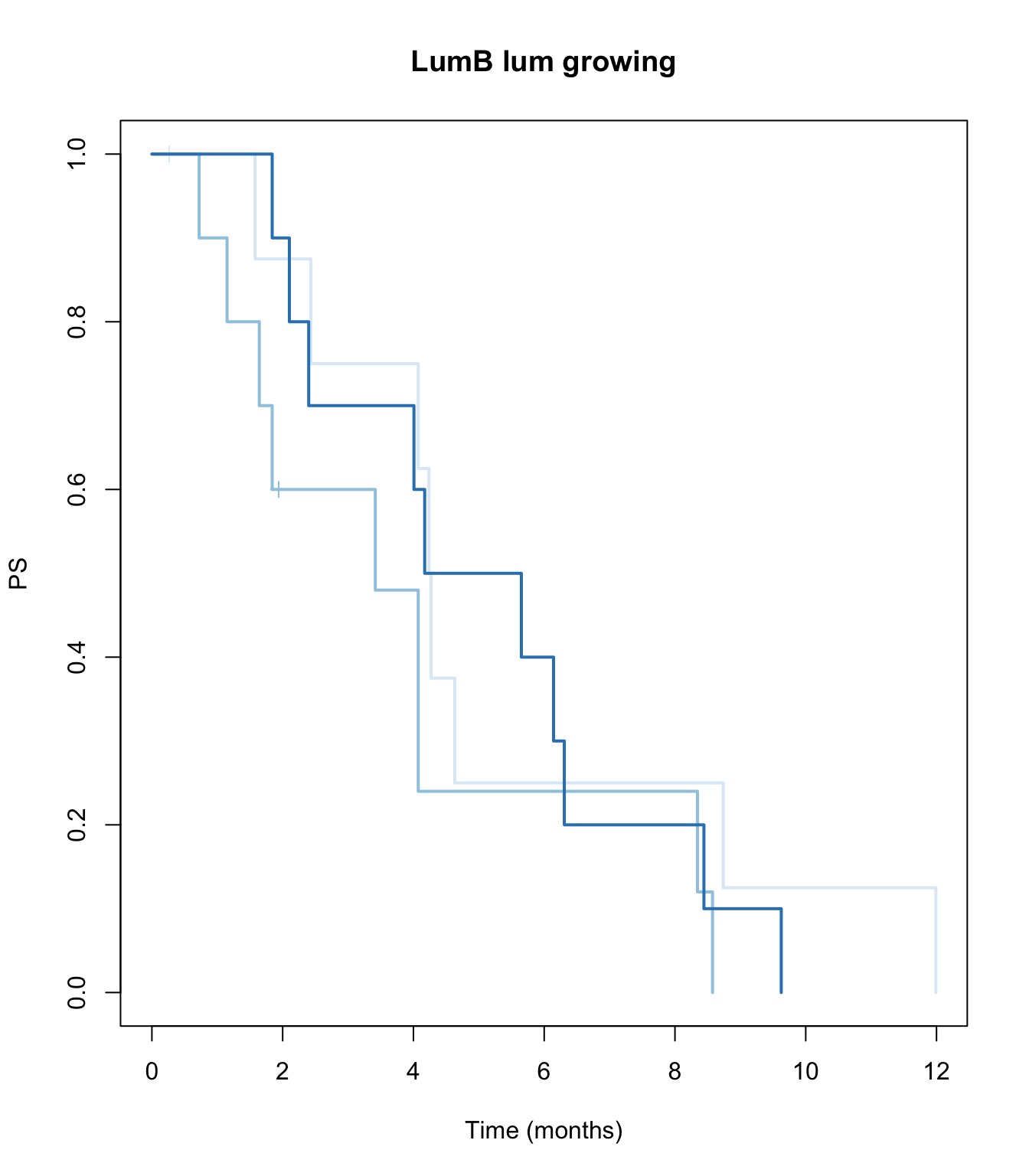
ax2=plot(survfit(ssOS~TCGAvalCut), main=paste(i, "lum growing"), col=brewer.pal(3, "Blues"),lwd=2, xlab="Time (months)", ylab="OS", mark.time=T)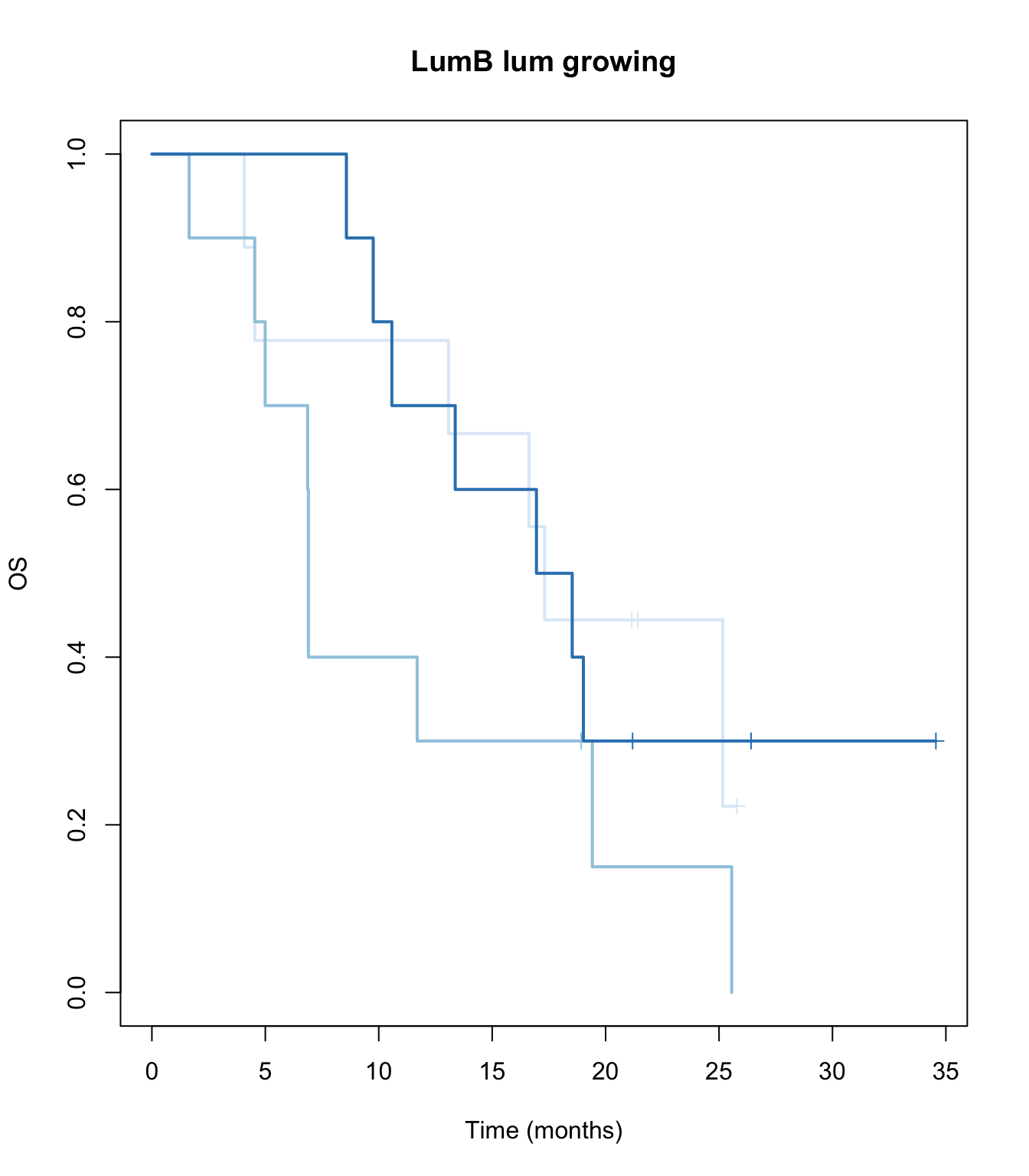
TCGAvalCut=cut(ERssgsea[2,ax3 ], quantile(ERssgsea[2,ax3], c(0, 0.33,0.67, 1)), c("L","M", "P"))

ax2=plot(survfit(ssPS~TCGAvalCut), main=paste(i, "lum stable"), col=brewer.pal(3, "Blues"),lwd=2, xlab="Time (months)", ylab="PS", mark.time=T)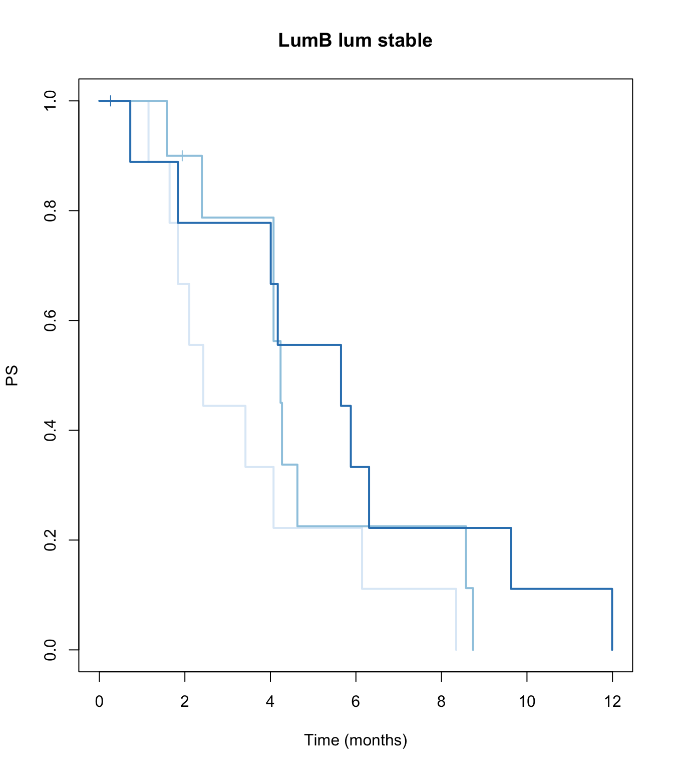
ax2=plot(survfit(ssOS~TCGAvalCut), main=paste(i, "lum stable"), col=brewer.pal(3, "Blues"),lwd=2, xlab="Time (months)", ylab="OS", mark.time=T)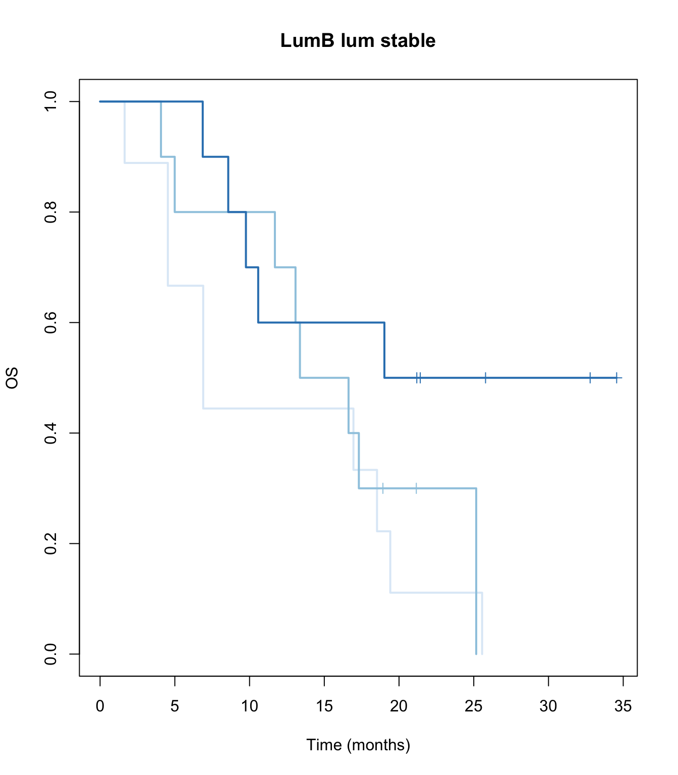
Run the above with Arm Stratification
aarm=which(ArmInfo=="A")
barm=which(ArmInfo=="B")
par(mfrow=c(1,2))
ax2=plot(survfit(ssPS[aarm]~TCGAvalCut[aarm]), main=paste(i, "lum growing Arm A"), col=brewer.pal(3, "Blues"),lwd=2, xlab="Time (months)", ylab="PS", mark.time=T)
ax2=plot(survfit(ssPS[barm]~TCGAvalCut[barm]), main=paste(i, "lum growing Arm B"), col=brewer.pal(3, "Blues"),lwd=2, xlab="Time (months)", ylab="PS", mark.time=T)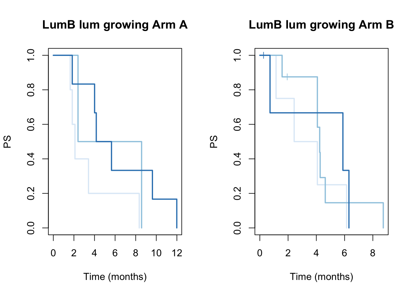
ax2=plot(survfit(ssOS[aarm]~TCGAvalCut[aarm]), main=paste(i, "lum growing"), col=brewer.pal(3, "Blues"),lwd=2, xlab="Time (months)", ylab="OS", mark.time=T)
ax2=plot(survfit(ssOS[barm]~TCGAvalCut[barm]), main=paste(i, "lum growing"), col=brewer.pal(3, "Blues"),lwd=2, xlab="Time (months)", ylab="OS", mark.time=T)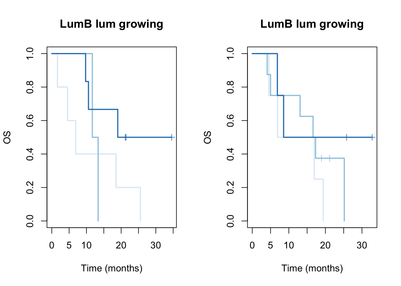
Also run the above as a continuous variable
## stable signature
ssPS=Surv( colDat$PFS.Months, colDat$Progression)
ssOS=Surv(colDat$OS.Months, colDat$Death )


dfs1=coxph(ssPS~ ERssgsea[1, ax3])
summary(dfs1)
## Call:
## coxph(formula = ssPS ~ ERssgsea[1, ax3])
##
##   n= 30, number of events= 28
##
##                       coef exp(coef)  se(coef)     z Pr(>|z|)
## ERssgsea[1, ax3] 0.0003460 1.0003461 0.0004729 0.732    0.464
##
##                  exp(coef) exp(-coef) lower .95 upper .95
## ERssgsea[1, ax3]         1     0.9997    0.9994     1.001
##
## Concordance= 0.532  (se = 0.06 )
## Likelihood ratio test= 0.54  on 1 df,   p=0.5
## Wald test            = 0.54  on 1 df,   p=0.5
## Score (logrank) test = 0.54  on 1 df,   p=0.5
dfs1=coxph(ssOS~ ERssgsea[1, ax3])
summary(dfs1)
## Call:
## coxph(formula = ssOS ~ ERssgsea[1, ax3])
##
##   n= 30, number of events= 22
##
##                       coef exp(coef)  se(coef)    z Pr(>|z|)
## ERssgsea[1, ax3] 0.0004201 1.0004202 0.0005525 0.76    0.447
##
##                  exp(coef) exp(-coef) lower .95 upper .95
## ERssgsea[1, ax3]         1     0.9996    0.9993     1.002
##
## Concordance= 0.511  (se = 0.07 )
## Likelihood ratio test= 0.59  on 1 df,   p=0.4
## Wald test            = 0.58  on 1 df,   p=0.4
## Score (logrank) test = 0.58  on 1 df,   p=0.4

## growing signature
dfs1=coxph(ssPS~ ERssgsea[2, ax3])
summary(dfs1)
## Call:
## coxph(formula = ssPS ~ ERssgsea[2, ax3])
##
##   n= 30, number of events= 28
##
##                        coef  exp(coef)   se(coef)      z Pr(>|z|)
## ERssgsea[2, ax3] -0.0002148  0.9997852  0.0001496 -1.436    0.151
##
##                  exp(coef) exp(-coef) lower .95 upper .95
## ERssgsea[2, ax3]    0.9998          1    0.9995         1
##
## Concordance= 0.597  (se = 0.07 )
## Likelihood ratio test= 1.94  on 1 df,   p=0.2
## Wald test            = 2.06  on 1 df,   p=0.2
## Score (logrank) test = 2.09  on 1 df,   p=0.1
dfs1=coxph(ssOS~ ERssgsea[2, ax3])
summary(dfs1)
## Call:
## coxph(formula = ssOS ~ ERssgsea[2, ax3])
##
##   n= 30, number of events= 22
##
##                        coef  exp(coef)   se(coef)      z Pr(>|z|)
## ERssgsea[2, ax3] -0.0001429  0.9998571  0.0001779 -0.803    0.422
##
##                  exp(coef) exp(-coef) lower .95 upper .95
## ERssgsea[2, ax3]    0.9999          1    0.9995         1
##
## Concordance= 0.58  (se = 0.074 )
## Likelihood ratio test= 0.61  on 1 df,   p=0.4
## Wald test            = 0.65  on 1 df,   p=0.4
## Score (logrank) test = 0.65  on 1 df,   p=0.4

## combined signature
dfs1=coxph(ssPS~(ERssgsea[2, ax3]-ERssgsea[1, ax3] ))
summary(dfs1)
## Call:
## coxph(formula = ssPS ~ (ERssgsea[2, ax3] - ERssgsea[1, ax3]))
##
##   n= 30, number of events= 28
##
##                        coef  exp(coef)   se(coef)      z Pr(>|z|)
## ERssgsea[2, ax3] -0.0002148  0.9997852  0.0001496 -1.436    0.151
##
##                  exp(coef) exp(-coef) lower .95 upper .95
## ERssgsea[2, ax3]    0.9998          1    0.9995         1
##
## Concordance= 0.597  (se = 0.07 )
## Likelihood ratio test= 1.94  on 1 df,   p=0.2
## Wald test            = 2.06  on 1 df,   p=0.2
## Score (logrank) test = 2.09  on 1 df,   p=0.1
dfs1=coxph(ssOS~ (ERssgsea[2, ax3]-ERssgsea[1, ax3] ))
summary(dfs1)
## Call:
## coxph(formula = ssOS ~ (ERssgsea[2, ax3] - ERssgsea[1, ax3]))
##
##   n= 30, number of events= 22
##
##                        coef  exp(coef)   se(coef)      z Pr(>|z|)
## ERssgsea[2, ax3] -0.0001429  0.9998571  0.0001779 -0.803    0.422
##
##                  exp(coef) exp(-coef) lower .95 upper .95
## ERssgsea[2, ax3]    0.9999          1    0.9995         1
##
## Concordance= 0.58  (se = 0.074 )
## Likelihood ratio test= 0.61  on 1 df,   p=0.4
## Wald test            = 0.65  on 1 df,   p=0.4
## Score (logrank) test = 0.65  on 1 df,   p=0.4