Chapter 4 Whole-slide imaging
In this section, we will be looking at the composition and spatial distribution of cells in whole slide images. These sections have previously been assessed using an external script: SpatialStatisticsWSI.R
The following markers have been used:
- EpCAM (tumor cells)
- SMA (fibroblasts or myeopithelial cells)
- CD8 (T cells)
Note that in some images a double positive EpCAM+/SMA+ population exists. Some CD8 cells have Epcam+ or SMA+ staining, however, we consider all of these to be simply CD8+
WSIpath="../data/WSI-data/locationData/"
WSIfiles=dir(WSIpath, "*.csv")
WSIsummary=lapply(WSIfiles, function(x) read.csv(paste(WSIpath, x, sep="")))
names(WSIsummary)=sapply(strsplit(WSIfiles, "_"), function(x) x[1])

## knn data
WSIpath="../data/WSI-data/knn-values/"
WSIfiles=dir(WSIpath, "*.csv")
WSIknn=lapply(WSIfiles, function(x) read.csv(paste(WSIpath, x, sep="")))
names(WSIknn)=sapply(strsplit(WSIfiles, "_"), function(x) x[1])

## knn data
WSIpath="../data/WSI-data/interactingFraction/"
WSIfiles=dir(WSIpath, "*.csv")
WSIIF=lapply(WSIfiles, function(x) read.csv(paste(WSIpath, x, sep="")))
WSIIF=lapply(WSIIF, function(x) {colnames(x)<-c("RN","Grid", "NearestNeighbor", "IF", "Reference"); x})
names(WSIIF)=sapply(strsplit(WSIfiles, "_"), function(x) x[1])

# MH data
WSIpath="../data/WSI-data/mh-values/"
WSIfiles=dir(WSIpath, "*.csv")
WSIMH=lapply(WSIfiles, function(x) read.csv(paste(WSIpath, x, sep="")))
names(WSIMH)=sapply(strsplit(WSIfiles, "_"), function(x) x[1])

# MH set-up summary
WSIpath="../data/WSI-data/MHset-upSummary/"
WSIfiles=dir(WSIpath, "*.csv")
WSIMHsetup=lapply(WSIfiles, function(x) read.csv(paste(WSIpath, x, sep="")))
names(WSIMHsetup)=sapply(strsplit(WSIfiles, "_"), function(x) x[1])

save(WSIsummary, WSIknn, WSIIF, WSIMH, WSIMHsetup, file=sprintf("outputs/WSI_raw_data%s.RData", Sys.Date()))
4.1 Associate the frequencies with other data types
UPDATE THE CIBERSORT INFORMATION.
Note there are 47 samples with imaging data. 33 of these samples have FACS data, manual counts and TIMER scores
Correlate the following information:
- “CD8.WSI”: CD8 total counts
- “CD8Frac.WSI”: CD8 fraction (normalised by cell count)
- “CD8_EPorSMARatio.WSI”: CD8/EP+SMA ratio (any EpCAM or SMA + cell)
- “CD8_AnySMARatio.WSI”: CD8/Any EPcam+ cell
- “CD8_EPRatio.WSI”: CD8 to EpCAM+SMA- ratio
- “CD8normTumSize”: normalised CD8 counts per mm of tumor size at sac
- “CD8.EpBoundingBox”: approx area per CD8 cell (density)
UPDATE THE CIBERSORT INFORMATION.
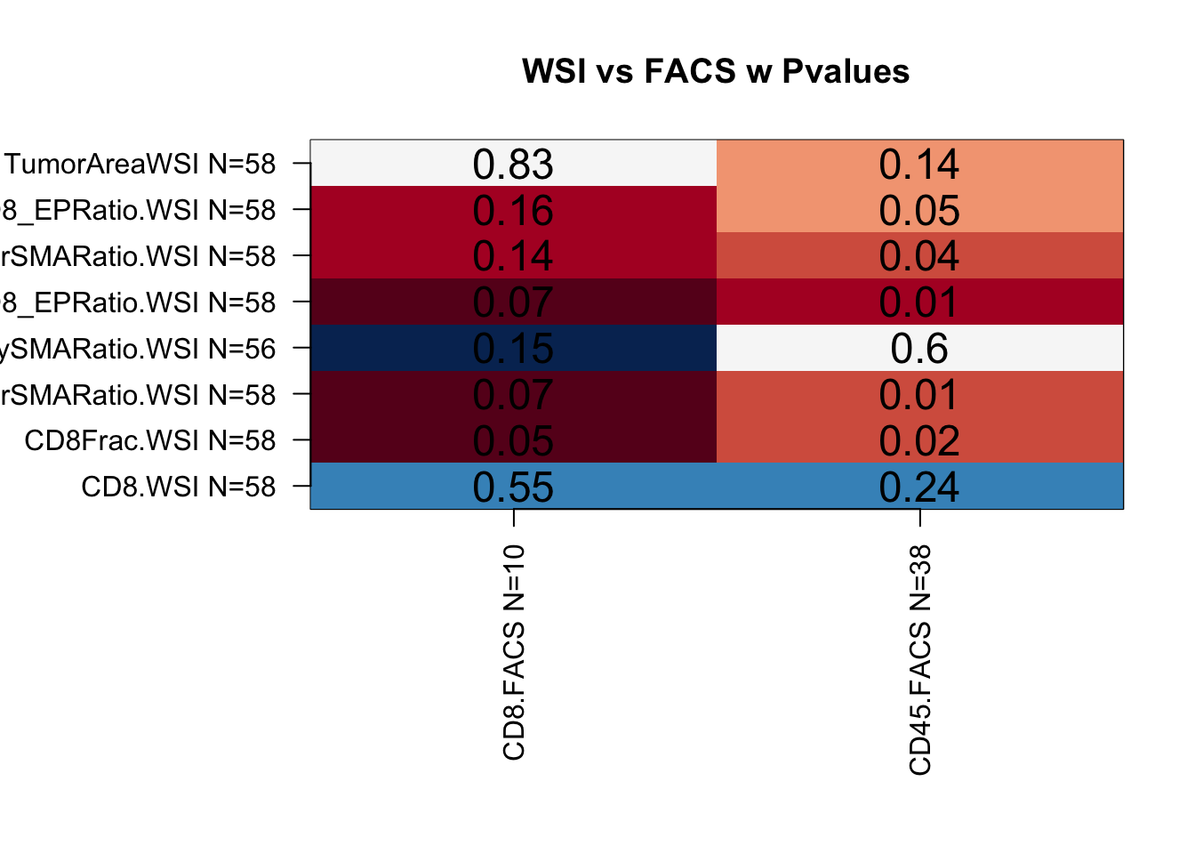
Below are heatmaps which show the correlation between two variables (red is correlated and blue is anti-correlated), and the p.value is indicated in the middle of the square.
It appears that CD8 whole-slide imaging associates well with:
- FACS data (both CD8 and CD45)
- Manual scoring (Fig 4) of CD8 cells
- Some CD8 gene signature scores (mainly in EPC, TIMER)
SummaryData=read.csv("../metadata/summary_final_210330.csv", row.names = 1)

## CD summary
NAidx=sapply(1:ncol(SummaryData), function(x) length(which(!is.na(SummaryData[, x]))))
names(NAidx)=colnames(SummaryData)

colTestCD8=c("CD8.EpBoundingBox", "CD45.FACS", "CD8.FACS", "OverallCD8_Fig4c.Manual", "TIL_Fig4d.Manual", "T.cell.CD8._TIMER", "T.cell.CD8._CIBERSORT","T.cell.CD8._CIBERSORT.ABS", "T.cell.CD8._EPIC")

# colTestCD8=c("CD8.EpDomTiles","CD8.EpBoundingBox", "CD8.TumSize", "CD45.FACS", "CD8.FACS", "OverallCD8_Fig4c.Manual", "TIL_Fig4d.Manual", )
indx1=c("CD8.WSI", "CD8Frac.WSI", "CD8_EPorSMARatio.WSI","CD8_AnySMARatio.WSI", "CD8_EPRatio.WSI","CD8normTumSize", "CD8.EpBoundingBox") #, "log2CD8_EPorSMARatio.WSI", "log2CD8_EPRatio.WSI")

CDsummary=matrix(NA, nrow=length(indx1), ncol=length(colTestCD8))
rownames(CDsummary)=paste(indx1, " N=", NAidx[match(indx1, names(NAidx))], sep="")
colnames(CDsummary)=paste(colTestCD8, " N=", NAidx[match(colTestCD8, names(NAidx))], sep="")
CDsummaryP=CDsummary
for (i in 1:length(indx1)){
  CDsummary[i, ]=sapply(colTestCD8, function(x) cor(SummaryData[, indx1[i]], SummaryData[,x], use="complete"))
  CDsummaryP[i, ]=sapply(colTestCD8, function(x) cor.test(SummaryData[, indx1[i]], SummaryData[,x], use="complete")$p.value)
}

## Do the same with EPCAM/FACS data

colTestFACS=grep("FACS", colnames(SummaryData), value = T)
colTestWSI=grep("WSI", colnames(SummaryData), value = T)
FACSsummary=matrix(NA, nrow=length(colTestFACS), ncol=length(colTestWSI))
rownames(FACSsummary)=paste(colTestFACS, " N=", NAidx[match(colTestFACS, names(NAidx))], sep="")
colnames(FACSsummary)=paste(colTestWSI, " N=", NAidx[match(colTestWSI, names(NAidx))], sep="")
FACSsummaryP=FACSsummary


for (i in 1:length(colTestFACS)){
  FACSsummary[i, ]=sapply(colTestWSI, function(x) cor(SummaryData[, colTestFACS[i]], SummaryData[,x], use="complete"))
  FACSsummaryP[i, ]=sapply(colTestWSI, function(x) cor.test(SummaryData[, colTestFACS[i]], SummaryData[,x], use="complete")$p.value)
}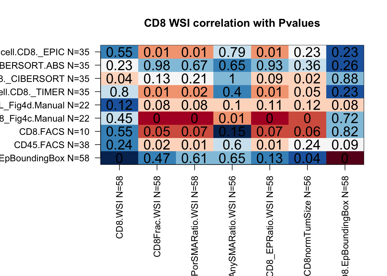
Figure 4.1: association with facs
4.2 Cellular composition
WSIvals=sapply(WSIsummary, function(x) table(factor(x$Class2, levels=c("CD8", "EpCAM", "EpCAM: SMA", "SMA", "Unclass"))))
WSIvalFracs=t(t(WSIvals)/colSums(WSIvals))

lxmatch=match(colnames(WSIvalFracs), gsub("_", "", Cdata$TumorID))

Cdata$CD8Fraction=NA
Cdata$CD8Fraction[na.omit(lxmatch)]=WSIvalFracs[1, ]

Cdata$EpCAMFraction=NA
Cdata$EpCAMFraction[na.omit(lxmatch)]=WSIvalFracs[2, ]

Cdata$DPFraction=NA
Cdata$DPFraction[na.omit(lxmatch)]=WSIvalFracs[3, ]

Cdata$SMAFraction=NA
Cdata$SMAFraction[na.omit(lxmatch)]=WSIvalFracs[4, ]

Cdata$UnclassFraction=NA
Cdata$UnclassFraction[na.omit(lxmatch)]=WSIvalFracs[5, ]

#write.csv(WSIvals, file="nature-tables/raw_WSI_values.csv")
#write.csv(WSIvalFracs, file="nature-tables/raw_WSI_values_fractions.csv")

df.Spatial=cbind(t(WSIvals), t(WSIvalFracs))
colnames(df.Spatial)=c("CD8", "EpCAM", "EpCAM:SMA", "SMA", "Unclass", paste(c("CD8", "EpCAM", "EpCAM:SMA", "SMA", "Unclass"), "frac", sep=""))

DT::datatable(df.Spatial, rownames=F, class='cell-border stripe',
          extensions="Buttons", options=list(dom="Bfrtip", buttons=c('csv', 'excel')))
Here, we look at the raw distributions of the different cell types and see if there are associations with:
- tumor size
- growth rate
- growth rate (categorical)
- treatment
- stromal restricted or infiltrating
Below are the total cell counts:
WSIvals=WSIvals[ , order(WSIvals[1, ])]
ordV=colnames(WSIvals)

WSIvalFracs=WSIvalFracs[ , order(WSIvalFracs[1, ])]
ordV2=colnames(WSIvalFracs)


## match with meta data# get the sample Names
CdataTID=gsub("_", "", Cdata$TumorID)
l1=match(colnames(WSIvals), CdataTID)
namesA=Cdata$NewID[l1]
###
Treat=Cdata$Treatment[l1]
Growth=Cdata$Growth2[l1]
WSImelt=melt(WSIvals)
#WSImelt$Var2=factor(WSImelt$Var2, levels=ordV)
WSImelt$treatment=Treat[match(WSImelt$Var2, colnames(WSIvals))]
WSImelt$growth=Growth[match(WSImelt$Var2, colnames(WSIvals))]
WSImelt$Name=namesA[match(WSImelt$Var2, colnames(WSIvals))]
WSImelt$Name=factor(WSImelt$Name, levels=namesA)

l2=match(colnames(WSIvalFracs), CdataTID)
namesA=Cdata$NewID[l2]
Treat=factor(Cdata$Treatment[l2])
Growth=Cdata$Growth2[l2]
WSIfracMelt=melt(WSIvalFracs)
#WSIfracMelt$Var2=factor(WSIfracMelt$Var2, levels=ordV2)
WSIfracMelt$treatment=Treat[match(WSIfracMelt$Var2, colnames(WSIvalFracs))]
WSIfracMelt$growth=Growth[match(WSIfracMelt$Var2, colnames(WSIvalFracs))]
WSIfracMelt$Name=namesA[match(WSIfracMelt$Var2, colnames(WSIvalFracs))]
WSIfracMelt$Name=factor(WSIfracMelt$Name, levels = namesA)


#pdf(sprintf("rslt/WSI-analysis/summary_distributions_norm_cell_count_%s.pdf", Sys.Date()), width=9, height=5)
ggplot(WSImelt, aes(x=Name, y=value, fill=Var1))+geom_bar(stat="identity")+theme(axis.text.x = element_text(angle = 90, hjust = 1))+ggtitle("ordered by CD8")
ggplot(WSImelt, aes(x=Name, y=value, fill=Var1))+geom_bar(stat="identity")+facet_grid(~treatment, space="free_x", scale="free_x")+theme(axis.text.x = element_text(angle = 90, hjust = 1))+ggtitle("ordered by treatment")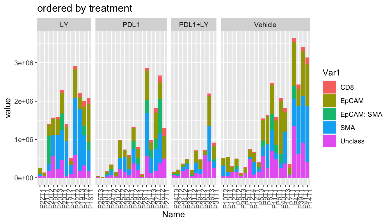
ggplot(WSImelt, aes(x=Name, y=value, fill=Var1))+geom_bar(stat="identity")+facet_grid(~growth, space="free_x", scale="free_x")+theme(axis.text.x = element_text(angle = 90, hjust = 1))+ggtitle("ordered by growth")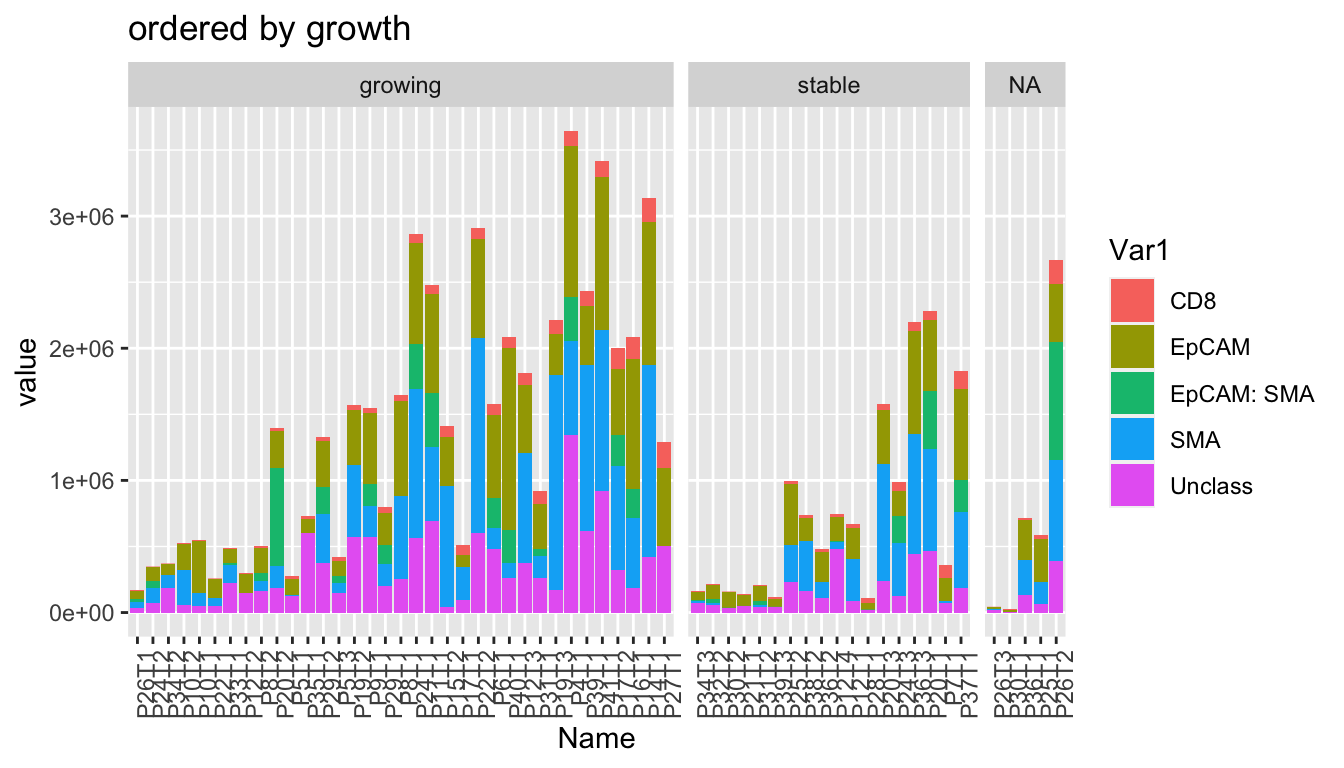
Here, the same data is shown and normalised according to total cell count:
pdf("figure-outputs/Fig4_WSI-normalised-all-samples.pdf", width=8, height=5)
ggplot(WSIfracMelt, aes(x=Name, y=value, fill=Var1))+geom_bar(stat="identity")+theme(axis.text.x = element_text(angle = 90, hjust = 1))+ggtitle("ordered by CD8")
dev.off()
## quartz_off_screen
## 2pdf("figure-outputs/Fig4_WSI-normalised-all-samples-treatment.pdf", width=8, height=5)
ggplot(WSIfracMelt, aes(x=Name, y=value, fill=Var1))+geom_bar(stat="identity")+facet_grid(~treatment, space="free_x", scale="free_x")+theme(axis.text.x = element_text(angle = 90, hjust = 1))+ggtitle("ordered by treatment")
dev.off()
## quartz_off_screen
## 2pdf("figure-outputs/Fig4_WSI-normalised-all-samples-growth2.pdf", width=8, height=5)
ggplot(WSIfracMelt, aes(x=Name, y=value, fill=Var1))+geom_bar(stat="identity")+facet_grid(~growth, space="free_x", scale="free_x")+theme(axis.text.x = element_text(angle = 90, hjust = 1))+ggtitle("ordered by growth")
dev.off()
## quartz_off_screen
## 2
DT::datatable(WSIfracMelt, rownames=F, class='cell-border stripe',
extensions="Buttons", options=list(dom="Bfrtip", buttons=c('csv', 'excel')))(#fig:Ext4c_pt2)association with growth
4.3 Associate composition with other covariates
Make Boxplots of the above data, and index samples according to growth or with treatment
#pdf("~/Desktop/Fig4B-summary-WSI-growth-treatment.pdf", height=7, width=7)

nx1=levels(WSIfracMelt$Var1)

nOut=sapply(nx1, function(x) wilcox.test(WSIfracMelt$value[WSIfracMelt$growth=="growing" & WSIfracMelt$Var1==x],WSIfracMelt$value[WSIfracMelt$growth=="stable" & WSIfracMelt$Var1==x])$p.value)

ggplot(WSIfracMelt[-which(is.na(WSIfracMelt$growth)), ], aes(x=Var1, y=value, col=factor(growth)))+geom_boxplot()+geom_point(position=position_jitterdodge(),alpha=0.3)+
  scale_color_manual(values=c(ColSize, "black"))+theme(axis.text.x = element_text(angle = 90, hjust = 1))+ggtitle("ordered by CD8")+theme_bw()+ggtitle(paste(names(nOut), round(nOut,2), collapse=" ;"))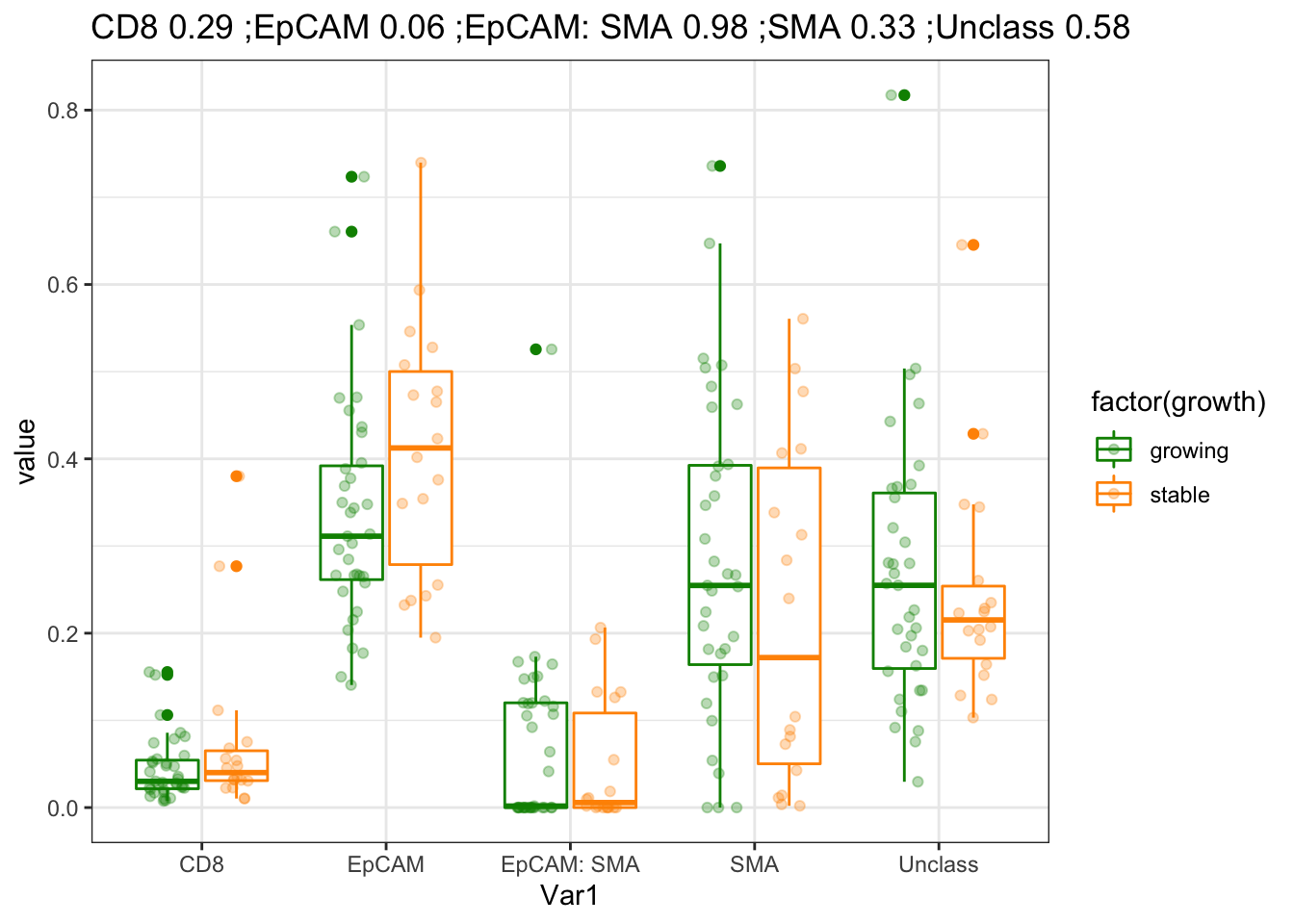
Figure 4.2: association of frequency with treatment and growth
nOutA=sapply(nx1, function(x) wilcox.test(WSIfracMelt$value[WSIfracMelt$treatment=="Vehicle" & WSIfracMelt$Var1==x],WSIfracMelt$value[WSIfracMelt$treatment=="LY" & WSIfracMelt$Var1==x])$p.value)

nOutB=sapply(nx1, function(x) wilcox.test(WSIfracMelt$value[WSIfracMelt$treatment=="Vehicle" & WSIfracMelt$Var1==x],WSIfracMelt$value[WSIfracMelt$treatment=="PDL1" & WSIfracMelt$Var1==x])$p.value)

nOutC=sapply(nx1, function(x) wilcox.test(WSIfracMelt$value[WSIfracMelt$treatment=="Vehicle" & WSIfracMelt$Var1==x],WSIfracMelt$value[WSIfracMelt$treatment=="PDL1+LY" & WSIfracMelt$Var1==x])$p.value)


ggplot(WSIfracMelt, aes(x=Var1, y=value, col=(treatment)))+geom_boxplot()+geom_point(position=position_jitterdodge(),alpha=0.3)+
  scale_color_manual(values=ColMerge[ ,1])+theme(axis.text.x = element_text(angle = 90, hjust = 1))+ggtitle("ordered by CD8")+theme_bw()+
  ggtitle(paste(paste(names(nOutA), round(nOutA,2), collapse=" ;"),paste(names(nOutB), round(nOutB,2), collapse=" ;"),paste(names(nOutC), round(nOutC,2), collapse=" ;") ) )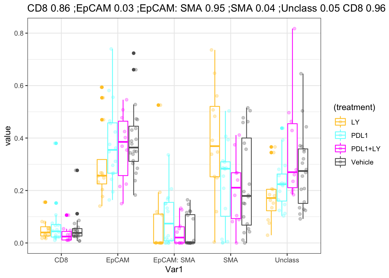
Figure 4.3: association with treatment
#dev.off()
DT::datatable(WSIfracMelt[-which(is.na(WSIfracMelt$growth)), ], rownames=F, class='cell-border stripe',
          extensions="Buttons", options=list(dom="Bfrtip", buttons=c('csv', 'excel')))
Figure 4.3: association with treatment
P values when comparing to the vehicle for each comparison:
| Treatment | values |
|---|---|
| LY | 0.8630663, 0.0323942, 0.9495167, 0.0437861, 0.04824 |
| PDL1 | 0.9624018, 0.6258328, 0.0255031, 0.9373764, 0.3049106 |
| PDL1+LY | 0.2307253, 1, 1, 0.9298782, 0.4479729 |
4.4 Estimate tumor size
Using WSI data, we can estimate a tumor size for each tissue sample and compare to the final tumor sizes. This will be based on the distribution of EpCAM+ cells. This estimate is can be used to normalise CD8 counts.
#estimate the tumor areas
Tarea=lapply(WSIsummary, function(x) ripras(x$Centroid.X.µm[x$Class2=="EpCAM"], x$Centroid.Y.µm[x$Class2=="EpCAM"], "convex"))
TareaSum=sapply(Tarea, area)

# Tumor diameter
Tdiameter=Cdata$Tumor.diameter.sac.mm[match(colnames(WSIvals), gsub("_", "", Cdata$TumorID))]

plot(TareaSum, Tdiameter, ylab="Tumor Diameter", xlab="Epcam cells bounding area")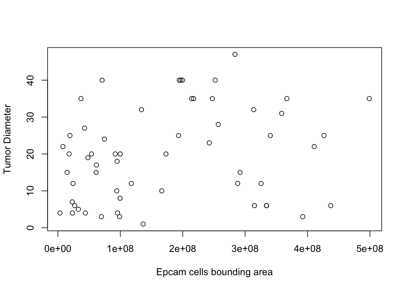
cor.test(TareaSum, Tdiameter, use="complete")
##
##  Pearson's product-moment correlation
##
## data:  TareaSum and Tdiameter
## t = 1.8547, df = 56, p-value = 0.06891
## alternative hypothesis: true correlation is not equal to 0
## 95 percent confidence interval:
##  -0.01890939  0.46967349
## sample estimates:
##       cor
## 0.2405613

## append to Cdata
Cdata$TumorAreaWSI=NA
lxmatch=match(colnames(WSIvalFracs), gsub("_", "", Cdata$TumorID)) # probably don't need this
Cdata$TumorAreaWSI[(lxmatch)]=TareaSum #[-which(is.na(lxmatch))]
4.5 Correlations between different subpopulations
Look for correlates between different subpopulations: Naturally, we would expect a negative correlation since this should sum to 1. Below are heatmaps showing correlations between different cell types, and significant associations are linearly shown.
Note the following negative correlations:
- epcam and SMA
- SMA+ and Unclass
Ax1=cor(t(WSIvalFracs))

#pdf(sprintf("rslt/WSI-analysis/summary-associations-between-subgroups_%s.pdf", Sys.Date()), height=8, width=8)
par(oma=c(4, 0,0, 4))
heatmap.2(Ax1, col=brewer.pal(9, "RdBu"), trace="none",scale="none")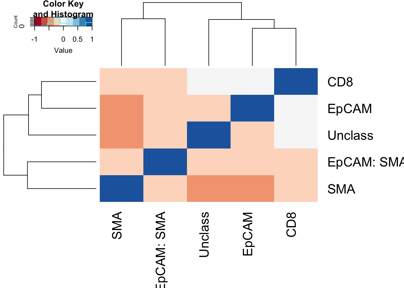
par(mfrow=c(2,2))

a1=cor.test(WSIvalFracs[2, ], WSIvalFracs[4, ])
plot(WSIvalFracs[2, ], WSIvalFracs[4, ], xlab="Epcam+", ylab="SMA+", main=sprintf("rho=%s,p=%s", round(a1$estimate, 2), round(a1$p.value, 2)))

a1=cor.test(WSIvalFracs[4, ], WSIvalFracs[5, ])
plot(WSIvalFracs[4, ], WSIvalFracs[5, ], xlab="SMA+", ylab="Unclass", main=sprintf("rho=%s,p=%s", round(a1$estimate, 2), round(a1$p.value, 2)))

a1=cor.test(WSIvalFracs[3, ], WSIvalFracs[4, ])
plot(WSIvalFracs[3, ], WSIvalFracs[4, ], xlab="Epcam+SMA+", ylab="SMA", main=sprintf("rho=%s,p=%s", round(a1$estimate, 2), round(a1$p.value, 2)))

a1=cor.test(WSIvalFracs[2, ], WSIvalFracs[5, ])
plot(WSIvalFracs[2, ], WSIvalFracs[5, ], xlab="Epcam+", ylab="nclass", main=sprintf("rho=%s,p=%s", round(a1$estimate, 2), round(a1$p.value, 2)))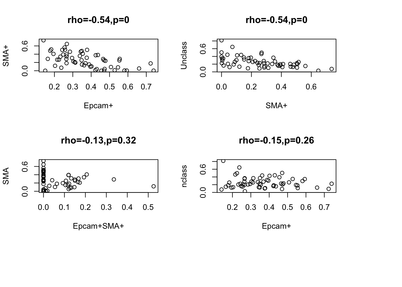
#devoff()

# correlations

ctest=matrix(NA, nrow=5, ncol=5)
for (i in 1:5){
  ctest[i, ]=sapply(1:5, function(x) cor.test(WSIvalFracs[i, ], WSIvalFracs[x, ])$p.value)
}
All associations determined using a correlation test
4.6 Associations between CD8 counts with other clinical variables
Below we assess whether any of the CD8-variables described in section 3.1 is associated with
- treatment
- growth
- spatial pattern
indx1=c(indx1, "log2CD8_EPorSMARatio.WSI", "log2CD8_EPRatio.WSI")

a1=matrix(NA, ncol=length(indx1), nrow=5)

for (i in 1:length(indx1)){
a1[1, i]=wilcox.test(SummaryData[SummaryData$Growth%in%c("stable", "growing") ,indx1[i] ]~ SummaryData$Growth[SummaryData$Growth%in%c("stable", "growing")])$p.value
a1[2, i]=wilcox.test(SummaryData[SummaryData$SpatialManual%in%c("Infiltrating", "restricted") ,indx1[i] ]~ SummaryData$SpatialManual[SummaryData$SpatialManual%in%c("Infiltrating", "restricted")])$p.value
a1[3, i]=wilcox.test(SummaryData[SummaryData$Treatment%in%c("PDL1", "Vehicle") ,indx1[i] ]~ SummaryData$Treatment[SummaryData$Treatment%in%c("PDL1", "Vehicle")])$p.value
a1[4, i]=wilcox.test(SummaryData[SummaryData$Treatment%in%c("PDL1+LY", "Vehicle") ,indx1[i] ]~ SummaryData$Treatment[SummaryData$Treatment%in%c("PDL1+LY", "Vehicle")])$p.value
a1[5, i]=wilcox.test(SummaryData[SummaryData$Treatment%in%c("LY", "Vehicle") ,indx1[i] ]~ SummaryData$Treatment[SummaryData$Treatment%in%c("LY", "Vehicle")])$p.value
}

colnames(a1)=indx1
rownames(a1)=c("growth", "spatial", "pdl1", "pdl1+ly", "ly")

par(oma=c(5, 0,0,4))
heatmap.2(-log10(a1), col=brewer.pal(9, "Blues"), trace="none", scale="none")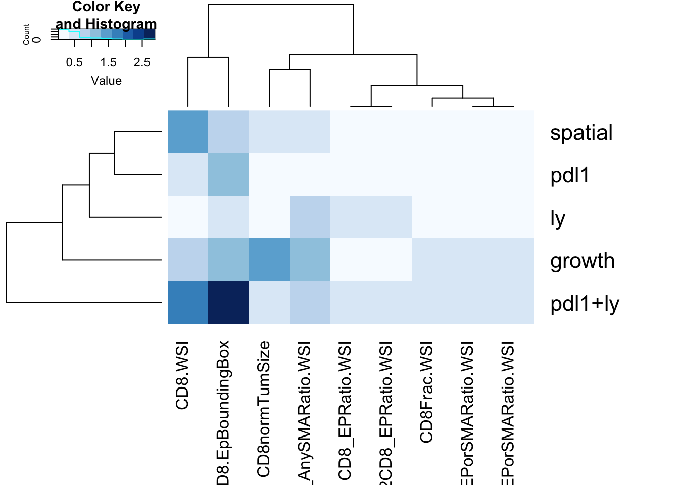
Note that CD8 normalised by tumor size is associated with growth (but this could a reflection of the size of the tumor), and there is a borderline difference once normalised by epithelial content. In addition the CD8 total count is associated with pdl1+ly treatment.
Note that p=0.05 is designated by a value of 1.3