Chapter 12 DESeq analysis: Immunotherapy/Growth comparisons
12.1 Summary of comparisons
Quick plot of the differences in number of differential genes:
Allchanges=rbind(UpDn1, CDUpDn1, DNUpDn1)
Allchanges=cbind(Allchanges, Frac=c("Ep", "Ep", "CD", "CD", "DN", "DN"), dir=rownames(Allchanges))
AllchangesB=melt(as.data.frame(Allchanges), id.vars = c("Frac", "dir"))
ggplot(AllchangesB, aes(x=variable, y=as.numeric(value), fill=dir))+geom_bar(stat="identity",position = "dodge")+facet_grid(Frac~., scale="free_y", space="free_y")+theme(axis.text.x = element_text(angle = 90, hjust = 1))+ylab("No. differential genes")+ggtitle("number of differential genes")+scale_y_log10()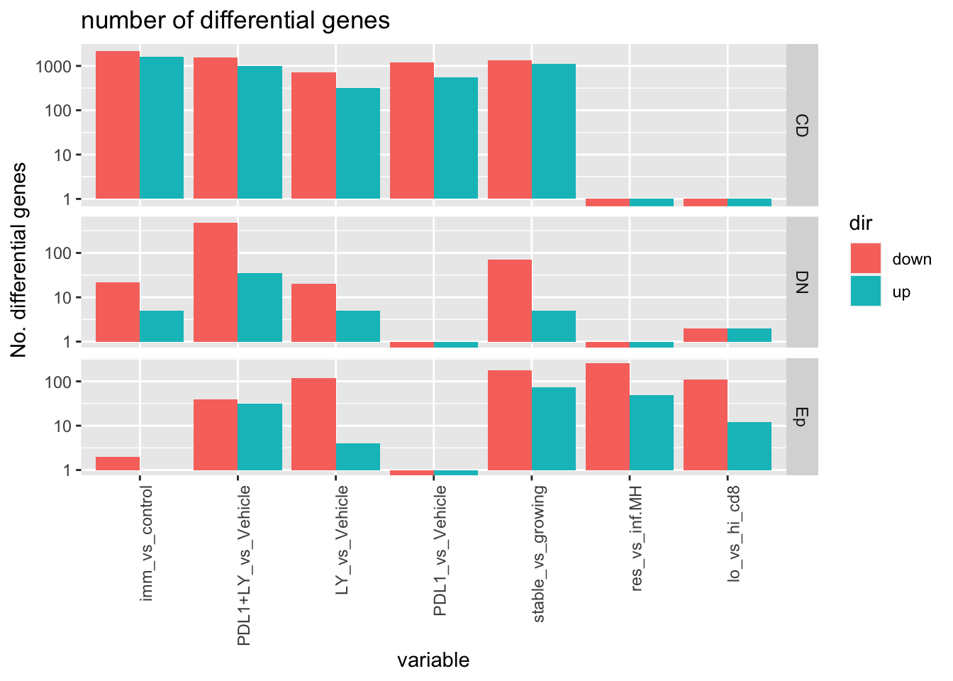
Notes:
| Comparison Type | Main cell type impacted |
|---|---|
| Treatment | CD45+, PDL1+LY in the DN, LY may affect Ep |
| growth | Ep and CD45 |
| growth in control | CD and DN |
| Spatial Patterns | CD45, Ep |
| Spatial, high cd8 | all cases |
12.2 DESeq: immunotherapy
What are the differential genes if we compare 1. All immunotherapy vs the control arm? 2. all pairwise comparisons: (each immunotherapy to the control arm?)
First look at the epithelial fraction:
# EpddsTreatB=EpddsTreat
# design(EpddsTreatB)=~treatA+factor(Batch)
# EpddsTreatB=DESeq(EpddsTreatB)
epr=results(Epdds)
Xa1=epr[which(epr$padj<0.05 & epr$baseMean>100), ]
epvsd=vst(Epdds)
assay(epvsd)<- limma::removeBatchEffect(assay(epvsd),factor(epvsd$Batch))
Mat2=epvsd[match(rownames(Xa1), rownames(epvsd)), ]
colSCols=ColMerge[ ,1][Mat2$Treatment]
heatmap.2(assay(Mat2), ColSideColors = colSCols, trace="none", scale="row", col=RdBu[11:1], hclustfun = hclust.ave)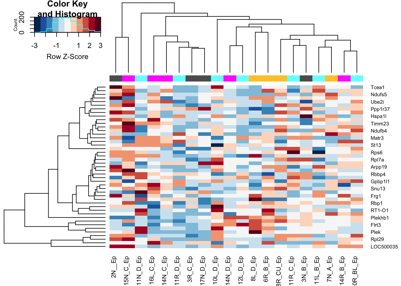
DT::datatable(as.data.frame(Xa1), rownames=T, class='cell-border stripe',
extensions="Buttons", options=list(dom="Bfrtip", buttons=c('csv', 'excel')))
## all pairwise comparisons:
ax1=results(EpddsTreat, c("Treatment", "LY", "Vehicle"))
bx1=results(EpddsTreat, c("Treatment", "PDL1", "Vehicle"))
cx1=results(EpddsTreat, c("Treatment", "PDL1+LY", "Vehicle"))
testout=cbind(ax1, bx1, cx1)
DT::datatable(as.data.frame(testout), rownames=T, class='cell-border stripe',
extensions="Buttons", options=list(dom="Bfrtip", buttons=c('csv', 'excel')))DN: two data tables are shown: first is any immunotherapy vs the vechicle. The second shows all pairwise comparisons in the order LY, PDL1, combo
xcellgenes=readxl::read_xlsx("../anntotations/xcell_genes.xlsx", sheet=1)
AllGenes=as.vector(xcellgenes[ ,-c(1:2)])
AllGenes=firstup(tolower(unique(as.character(unlist(AllGenes)))))
#rm list
rmList=c("15L_B_DN", "6R_B_DN", "10L_C_DN", "6R_D_DN")
DNr=results(DNdds)
Xa1=DNr[which(DNr$padj<0.05 & DNr$baseMean>100 & abs(DNr$log2FoldChange)>1.5), ]
# DNvsd=vst(DNddsTreatB)
# assay(DNvsd)<- limma::removeBatchEffect(assay(DNvsd),factor(DNvsd$Batch))
AllG2=rownames(Xa1)[which(rownames(Xa1)%in%c(AllGenes, "Il6"))]
Mat2=vsdLimmaDN[match(AllG2, rownames(vsdLimmaDN)), ]
colnames(Mat2)=Cdata$NewID[match(substr(colnames(Mat2),1 , nchar(colnames(Mat2))-3), Cdata$TumorID)]
colSCols=ColMerge[ ,1][Mat2$Treatment]
heatmap.2(assay(Mat2), ColSideColors = colSCols, trace="none", scale="row", col=RdBu[11:1])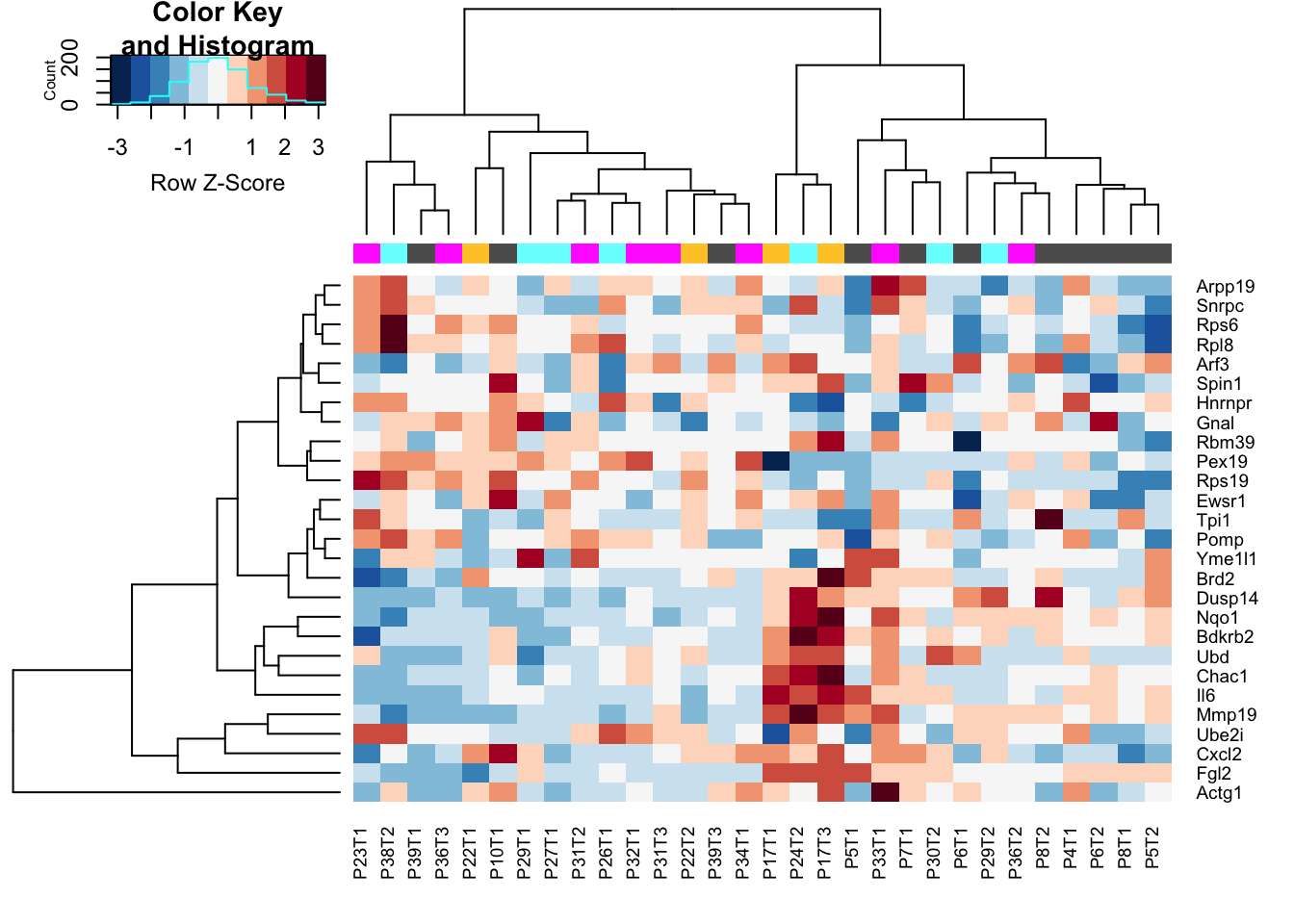
DT::datatable(as.data.frame(Xa1), rownames=T, class='cell-border stripe',
extensions="Buttons", options=list(dom="Bfrtip", buttons=c('csv', 'excel')))
#write.csv(DNr, file="nature-tables/Supp2_DN_io_vs_non_io.csv")
ax1=results(DNddsTreat, c("Treatment", "LY", "Vehicle"))
bx1=results(DNddsTreat, c("Treatment", "PDL1", "Vehicle"))
cx1=results(DNddsTreat, c("Treatment", "PDL1+LY", "Vehicle"))
testout=cbind(ax1, bx1, cx1)
DT::datatable(as.data.frame(testout), rownames=T, class='cell-border stripe',
extensions="Buttons", options=list(dom="Bfrtip", buttons=c('csv', 'excel')))CD45: three data tables are shown: first are values used in the heatmap second is any immunotherapy vs the vechicle. third shows all pairwise comparisons in the order LY, PDL1, combo
# CDddsTreatB=CDddsTreat
# design(CDddsTreatB)=~treatA
# CDddsTreatB=DESeq(CDddsTreatB)
CDr=results(CDdds)
Xa1=CDr[which(CDr$padj<0.05 & CDr$baseMean>100 & abs(CDr$log2FoldChange)>1.5), ]
AllG2=rownames(Xa1)[which(rownames(Xa1)%in%RatAllImm)]
Mat2=vsdLimmaCD[match(AllG2, rownames(vsdLimmaCD)), ]
colnames(Mat2)=Cdata$NewID[match(substr(colnames(Mat2),1 , nchar(colnames(Mat2))-5), Cdata$TumorID)]
colSCols=ColMerge[ ,1][Mat2$Treatment]
#pdf("figure-outputs/FIgure3j_1_vs_all.pdf", height=7, width=6)
heatmap.2(assay(Mat2), ColSideColors = colSCols, trace="none", scale="row", col=RdBu[11:1],
hclustfun = hclust.ave)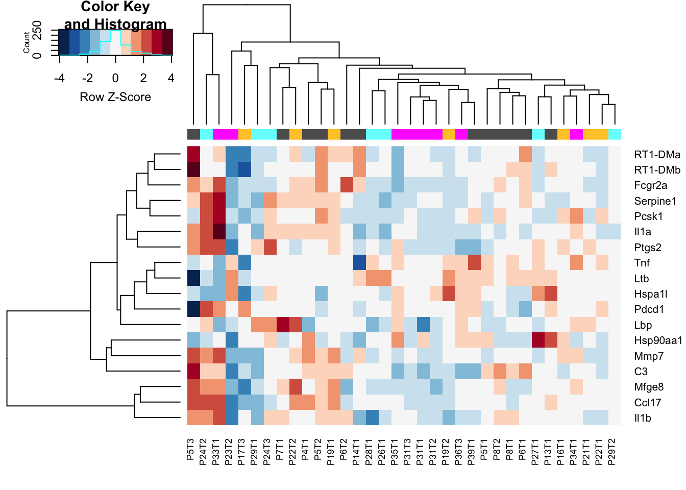
Figure 12.1: CD45 IO vs non-IO
#dev.off()
#DT::datatable(as.data.frame(Mat2), rownames=F, class='cell-border stripe',
# extensions="Buttons", options=list(dom="Bfrtip", buttons=c('csv', 'excel')))
#write.csv(assay(Mat2), file="nature-tables/Figure3j_1_vs_all.csv")
DT::datatable(as.data.frame(CDr), rownames=T, class='cell-border stripe',
extensions="Buttons", options=list(dom="Bfrtip", buttons=c('csv', 'excel')))Figure 12.1: CD45 IO vs non-IO
## ALSO LOOK AT the pairwise comparisons and pull out those genes
ax1=results(CDddsTreat, c("Treatment", "LY", "Vehicle"))
bx1=results(CDddsTreat, c("Treatment", "PDL1", "Vehicle"))
cx1=results(CDddsTreat, c("Treatment", "PDL1+LY", "Vehicle"))
xa=rownames(ax1)
xb=rownames(bx1)
xc=rownames(cx1)
G1=rownames(ax1)[which(ax1$baseMean>100 & ax1$padj<0.05 & abs(ax1$log2FoldChange)>1.5)]
G2=rownames(bx1)[which(bx1$baseMean>100 & bx1$padj<0.05 & abs(bx1$log2FoldChange)>1.5)]
G3=rownames(cx1)[which(cx1$baseMean>100 & cx1$padj<0.05 & abs(cx1$log2FoldChange)>1.5)]
AllG=unique(c(G1, G2, G3))
AllG2=AllG[which(AllG%in%RatAllImm)]
Mat2=vsdLimmaCD[match(AllG2, rownames(vsdLimmaCD)), ]
colnames(Mat2)=Cdata$NewID[match(substr(colnames(Mat2),1 , nchar(colnames(Mat2))-5), Cdata$TumorID)]
colSCols=ColMerge[ ,1][Mat2$Treatment]
#pdf("figure-outputs/FIgure3j_all_comparisons.pdf", height=9, width=6)
heatmap.2(assay(Mat2), ColSideColors = colSCols, trace="none", scale="row", col=RdBu[11:1], hclustfun = hclust.ave)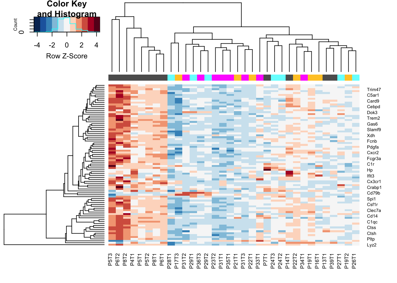
Figure 12.2: IO vs any other treatment
#dev.off()
testout=cbind(ax1, bx1, cx1)
DT::datatable(as.data.frame(testout), rownames=T, class='cell-border stripe',
extensions="Buttons", options=list(dom="Bfrtip", buttons=c('csv', 'excel')))Figure 12.2: IO vs any other treatment
12.3 Growing vs stable emphasis
Below, we focus specifically on the growing vs stable comparison in greater depth. Here, we look at the 3 different fractions in greater depth and look at volcano plots of DEG and heatmaps of differential genes. Samples are colored according to whether they are growing or stable
12.3.1 DN fraction
#pdf(sprintf("rslt/DESeq/volcano_plots_differences_stable_vs_growing_%s.pdf", Sys.Date()), height=7, width=8)
DNa1=results(DNddsGrowth,contrast=c("Growth", "stable", "growing")) #DNComp4$stable_vs_growing
DNa1$Gene=rownames(DNa1)
DNa=DNa1[ which(DNa1$padj<0.05 & DNa1$baseMean>100 & abs(DNa1$log2FoldChange)>1.5), ]
with(DNa1, plot(log2FoldChange, -log10(padj), pch=20, main="Volcano plot: DN growing (+) vs stable (-)", cex=1.0, xlab=bquote(~Log[2]~fold~change), ylab=bquote(~-log[10]~Q~value)))
with(subset(DNa1, padj<0.05 & abs(log2FoldChange)>1.5 & baseMean>100), points(log2FoldChange, -log10(padj), pch=20, col="red", cex=0.5))
with(subset(DNa1, padj<0.05 & abs(log2FoldChange)>1.5 & baseMean>100), text(log2FoldChange+0.05, -log10(padj)+0.05, Gene, pch=20, col="red", cex=0.75))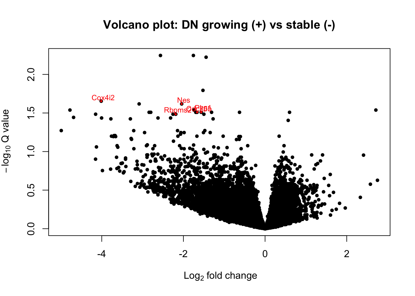
vstDN$GRcutoff=cut(vstDN$GrowthRate, c(-1, 2, 5, 10, 20), c("L", "M1", "O1", "O2") )
colnames(vstDN)=vstDN$TumorIDnew
heatmap.2(assay(vstDN)[ DNa$Gene, ], scale="row", trace="none", ColSideColors =brewer.pal(4, "Greens")[ (as.numeric(factor(vstDN$GRcutoff)))], col=RdBu[11:1], main="DN genes")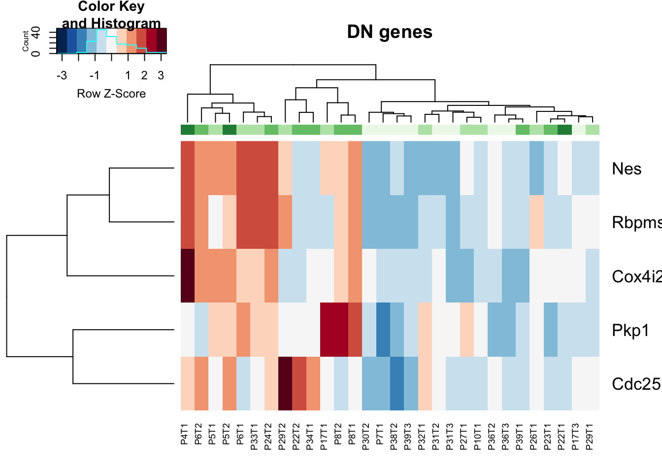
12.3.2 CD fraction
Volcano plot
#pdf("~/Desktop/Figure4G_CD_stable_growing.pdf", height=12, width=12)
CDa1=results(CDddsGrowth, contrast=c("Growth", "stable", "growing"))
CDa1$Gene=rownames(CDa1)
#CDa1=CDComp4$stable_vs_growing
CDa=CDa1[ which(CDa1$padj<0.05 & CDa1$baseMean>100 & abs(CDa1$log2FoldChange)>1.5), ]
lx2=which(CDa$Gene%in%RatAllImm)
with(CDa1, plot(log2FoldChange, -log10(padj), pch=20, main="Volcano plot: CD Stable (-) vs Growing (+)", cex=1.0, xlab=bquote(~Log[2]~fold~change), ylab=bquote(~-log[10]~Q~value)))
with(subset(CDa1, padj<0.05 & abs(log2FoldChange)>1.5 & baseMean>100 ), points(log2FoldChange, -log10(padj), pch=20, col="red", cex=0.5))
with(subset(CDa1, padj<0.05 & abs(log2FoldChange)>1.5 & baseMean>100 ), text(log2FoldChange+0.02, -log10(padj)+0.05, Gene, pch=20, col="red", cex=0.75))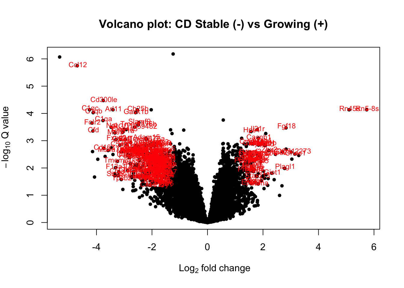
Figure 12.3: volcano plot of DEG stable vs growing CD45
#write.csv(CDa1, file="nature-tables/4g.csv")
DT::datatable(as.data.frame(CDa), rownames=T, class='cell-border stripe',
extensions="Buttons", options=list(dom="Bfrtip", buttons=c('csv', 'excel')))Figure 12.3: volcano plot of DEG stable vs growing CD45
Here are a bunch of heatmaps, which are then separated by wehther genes are downregulated (growing specific) or upregulated (stable specific)
vstCD$GRcutoff=cut(vstCD$GrowthRate, c(-1, 2, 5, 10, 20), c("L", "M1", "O1", "O2") )
colnames(vstCD)=vstCD$TumorIDnew
heatmap.2(assay(vstCD)[ CDa$Gene[lx2], ], scale="row", trace="none", ColSideColors =brewer.pal(4, "Greens")[ (as.numeric(factor(vstCD$GRcutoff)))], col=RdBu[11:1], main="CD genes")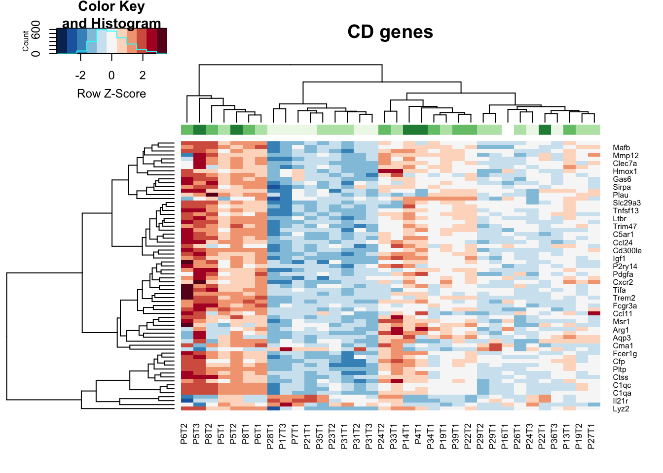
## growing specific
CDg=CDa$Gene[which(CDa$log2FoldChange<0)]
heatmap.2(assay(vstCD)[CDg, ], scale="row", trace="none", ColSideColors = as.character(as.numeric(vstCD$Growth)), col=RdBu[11:1], main="CD genes growing")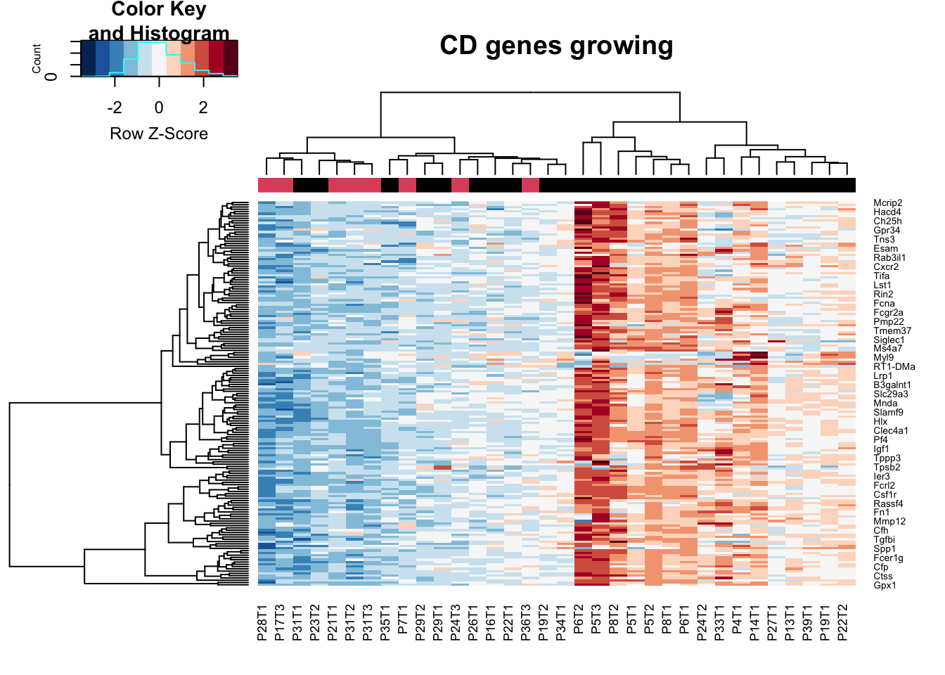
## stable specific
CDs=CDa$Gene[which(CDa$log2FoldChange>0)]
heatmap.2(assay(vstCD)[CDs, ], scale="row", trace="none", ColSideColors = as.character(as.numeric(vstCD$Growth)), col=RdBu[11:1], main="CD genes stable")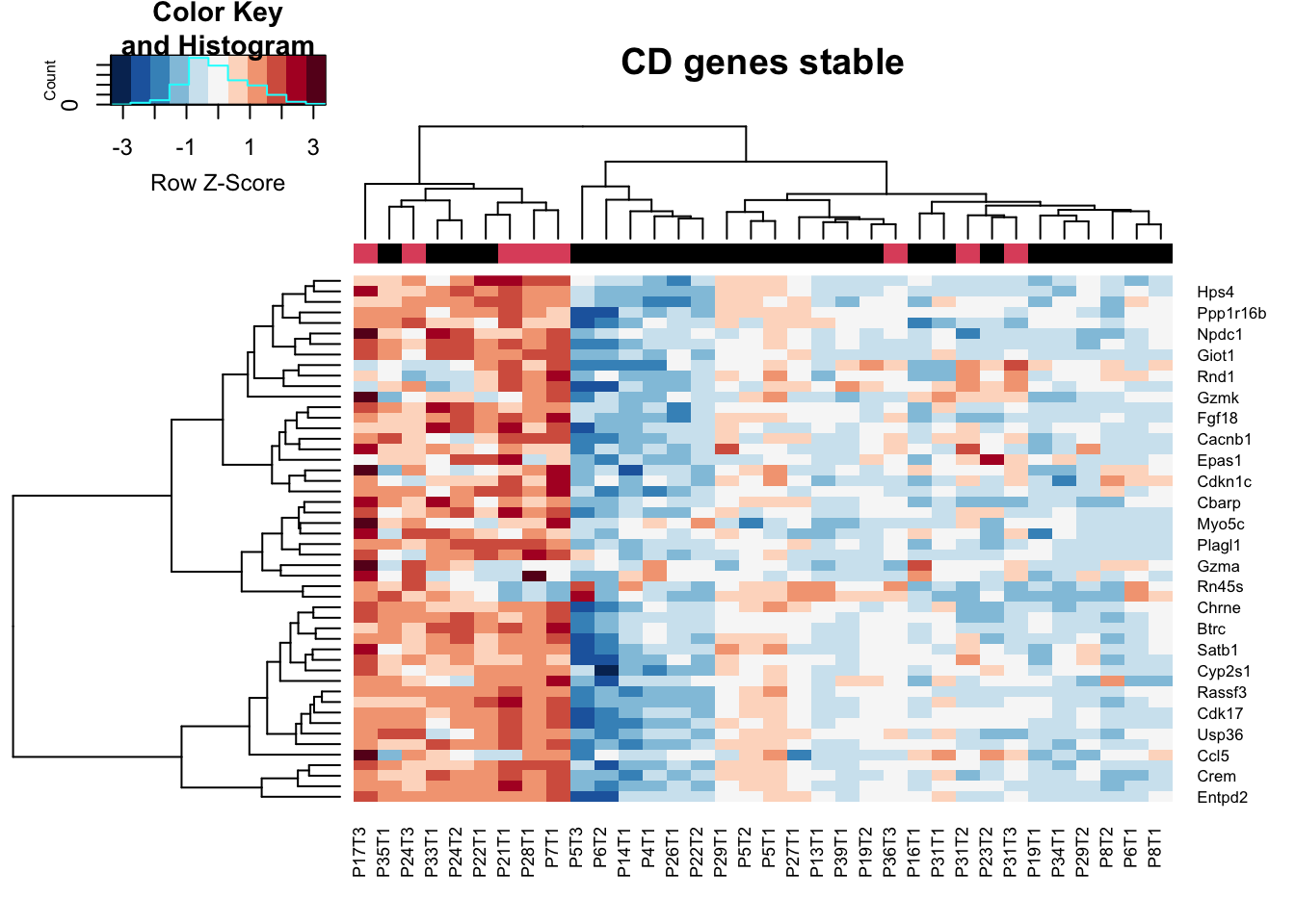
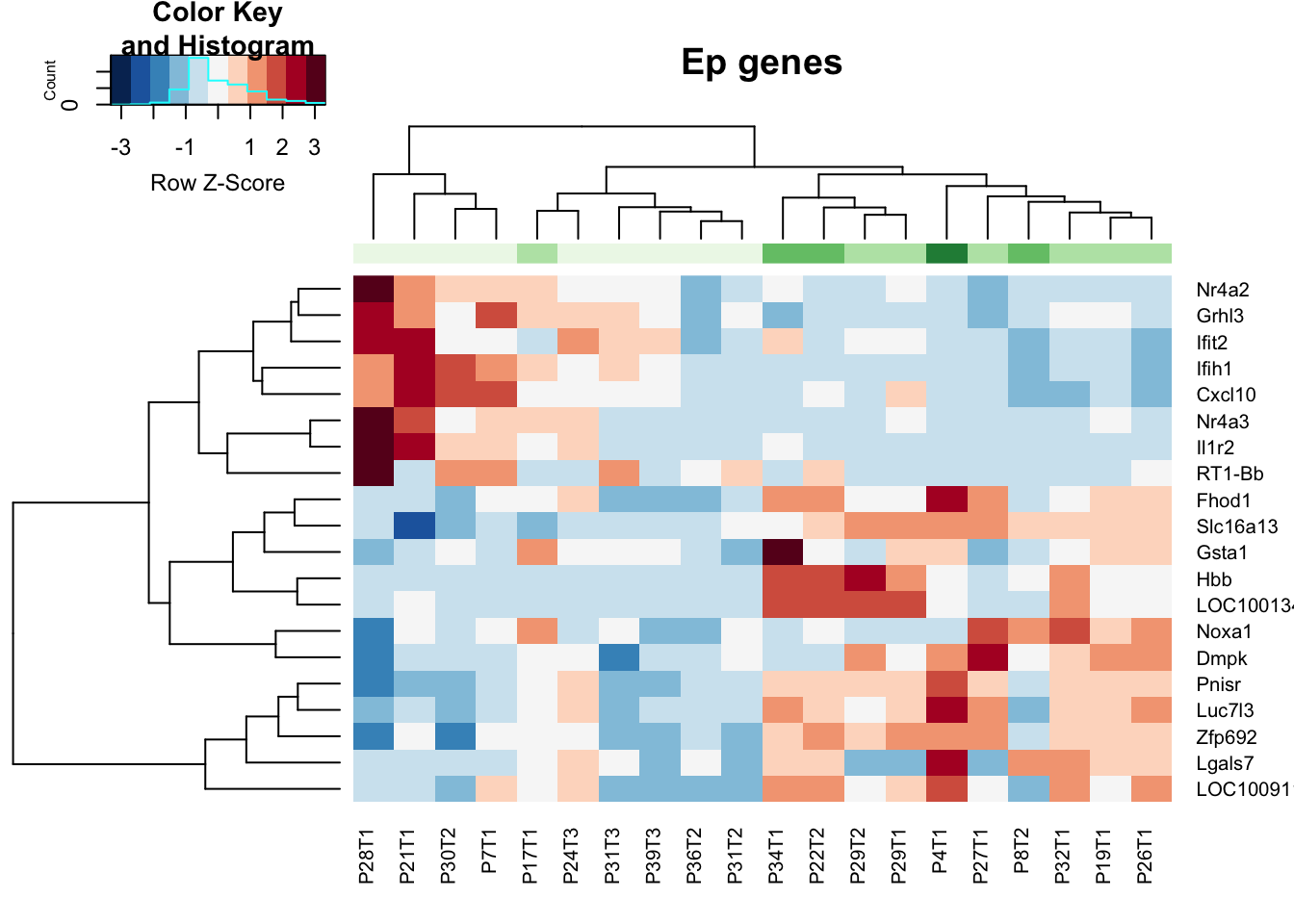
12.3.3 Ep Fraction
#Epa1=EpComp4$stable_vs_growing
Epa1=results(EpddsGrowth, contrast=c("Growth", "stable", "growing"))
Epa1$Gene=rownames(Epa1)
Epa=Epa1[ which(Epa1$padj<0.05 & Epa1$baseMean>100 & abs(Epa1$log2FoldChange)>1.5), ]
with(Epa1, plot(log2FoldChange, -log10(padj), pch=20, main="Volcano plot: Ep Stable (-) vs Growing (+)", cex=1.0, xlab=bquote(~Log[2]~fold~change), ylab=bquote(~-log[10]~Q~value)))
with(subset(Epa1, padj<0.05 & abs(log2FoldChange)>1.5), points(log2FoldChange, -log10(padj), pch=20, col="red", cex=0.5))
with(subset(Epa1, padj<0.05 & abs(log2FoldChange)>1.5), text(log2FoldChange+0.05, -log10(padj)+0.1, Gene, pch=20, col="red", cex=0.75))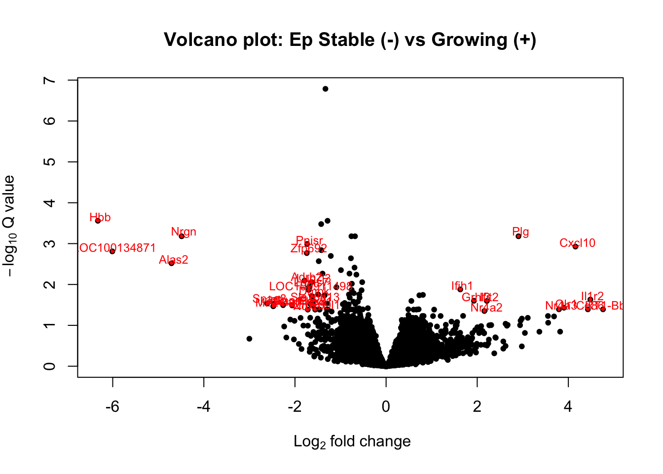
vstEp$GRcutoff=cut(vstEp$GrowthRate, c(-1, 2, 5, 10, 20), c("L", "M1", "O1", "O2") )
colnames(vstEp)=vstEp$TumorIDnew
#EpaB=Epa[order(1/abs(Epa$log2FoldChange), Epa$padj), ]
a1=dim(Epa)
heatmap.2(assay(vstEp)[ Epa$Gene, ], scale="row", trace="none", ColSideColors = brewer.pal(4, "Greens")[ (as.numeric(factor(vstEp$GRcutoff)))], col=RdBu[11:1], main="Ep genes")